Task
Compute values to be used as expected returns. A real process to create expected returns will of course be proprietary and presumably not a simple calculation.
But we simplify this here by changing the task to computing some technical indicator.
Preparation
- matrix of asset prices (or possibly returns)
You need a history of prices for the assets in the universe. Some indicators may use returns rather than prices.
Doing the example
pprobeDatapackageTTRpackage
You need to have the packages loaded into your R session:
require(pprobeData)
require(TTR)
If either is not installed on your machine, see “Using R packages”.
Doing it
In this example we compute the (default) MACD signal from the TTR package.
This is used as a handy example — it is not an endorsement of using it to manage money.
The first thing is to create an object the same size as the price matrix that has the same row and column names:
xaMACD <- xassetPrices
xaMACD[] <- NA
As a safety precaution, all the items in the matrix are changed to missing values.
The real work is done in the next command where the object we just created is filled with values, one column at a time.
for(i in 1:ncol(xaMACD)) {
   xaMACD[,i] <- MACD(xassetPrices[,i])[,"signal"]
}
Explanation
The signal we are getting is a somewhat complicated function of the usual MACD, which itself depends on two parameters. See the TTR documentation for details if you care.
Check your work
An easy thing to get wrong in experiments is that the predictor uses future data.
Here we will test to make sure that we are not using future data by modifying a small price series to have a large jump.
testp <- xassetPrices[1:100, 1]
At this point we merely have a price series that is 100 long. Now we add a big number to elements 75 through 100:
> tail(testp)
2006-05-18 2006-05-19 2006-05-22 2006-05-23
     23.92      24.06      24.30      24.27
2006-05-24 2006-05-25
     24.08      24.18
> testp[75:100] <- testp[75:100] + 100
We get our indicator on the modified series:
testSig <- MACD(testp)[,"signal"]
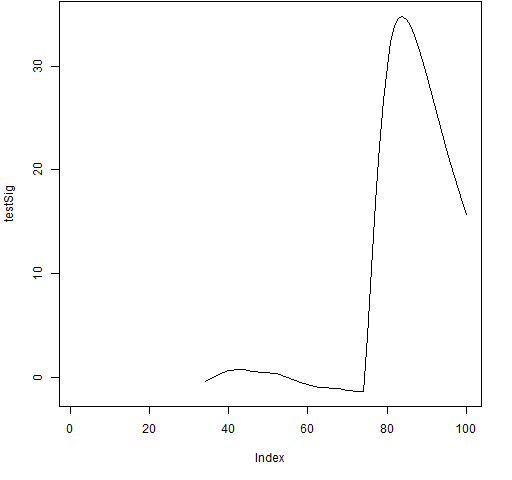
We plot the signal.
plot(testSig, type="l") # Figure 1
Figure 1: MACD signal on modified test data. 
We look at the range of values for the signal in the unmodified data, the first few results with the leap, and the last few before the leap:
> summary(testSig[1:74])
   Min. 1st Qu.  Median    Mean 3rd Qu.    Max.
-1.3770 -1.0170 -0.1907 -0.2459  0.4513  0.7387
   NA's
     33
> testSig[75:78]
2006-04-20 2006-04-21 2006-04-24 2006-04-25
  3.904804  10.496282  16.839948  22.306100
> testSig[71:74]
2006-04-13 2006-04-17 2006-04-18 2006-04-19
 -1.302102  -1.354493  -1.377073  -1.359459
Clearly the signal starts changing at element 75 which is where the jump is, and hence what we want.
Troubleshooting
- Do not misspell the name of the column to be extracted.
> for(i in 1:ncol(xaMACD)) {
+    xaMACD[,i] <- MACD(xassetPrices[,i])[,"Signal"]
+ }
Error: subscript out of bounds
The name is really "signal" and not "Signal" (capitalization matters).
Whenever there is an error in R, you can look at the traceback:
> traceback()
No traceback available
That there is no traceback means that the error is at the top level. There are three subscripts at the top level. The last one is the most likely to be the problem (and actually is).
Navigate
- Back to “Optimize Trades”
- Back to the top level of “Portfolio Probe Cookbook”
