Task
Compute the returns for a set of random portfolios over one or more time periods, compute the realized volatility, and do some plotting.
Preparation
This presumes that you can create a random portfolio object. For example, that you have mastered either “Very simple long-only” or “Very simple long-short”.
- random portfolio object
- Portfolio Probe
You need a random portfolio object with which to create valuations.
You also need to have the Portfolio Probe package loaded into your R session:
require(PortfolioProbe)
If you don’t have Portfolio Probe, see “Demo or Buy”.
Doing the example
rploVerysimpobject from the “Very simple long-only” examplepprobeDatapackage
You need to have the package loaded into your R session:
require(pprobeData)
Doing it
We do these tasks:
- compute the returns for a random portfolio object
- get the realized volatility of the random portfolios
- plot the density of the returns over one period
Compute the returns for a random portfolio object
We give the valuation function a price matrix that covers the period in which we are interested, and we specify which type of returns we want (the default is, of course, to return valuations rather than returns):
retDaily07 <- valuation(rploVerysimp,
   xassetPrices[251:502,], returns="log")
The prices given are the daily closing prices during 2007.
The result is a matrix that is the number of time points by the number of random portfolios:
> dim(retDaily07)
[1] 251   4
Get the realized volatility of the random portfolios
Now that we have returns for the random portfolios, we can compute their realized volatility over that time frame.
Volatility is merely the annualized standard deviation (and often expressed in percent):
volDaily07 <- apply(retDaily07, 2, sd) * sqrt(252) * 100
The result is:
> volDaily07
[1] 25.60307 18.68255 22.22142 29.25868
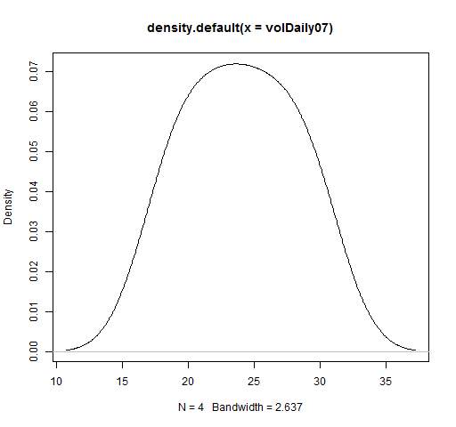
We can plot the distribution of the volatilities. Of course the plot is more sensible when there are a lot of volatilities.
The command to do such a plot is:
plot(density(volDaily07)) # Figure 1
Figure 1: Density of realized volatility.  See below for some tricks to get a prettier picture.
Plot distribution of returns
We want to get the simple returns for the entire year of 2007 for our random portfolios. The command to do that is:
sretAnn07 <- valuation(rploVerysimp,
   xassetPrices[c(251, 502),], returns="simple")
There are two small changes from the creation of retDaily07 above. The row subscript of the prices matrix changes from ‘251:502‘ to ‘c(251, 502)‘. The colon operator gives us all the integers from 251 to 502 while we get just the extremes with the second version. With this second version we get just one return for each random portfolio.
The other change is of course that we are asking for simple returns instead of log returns.
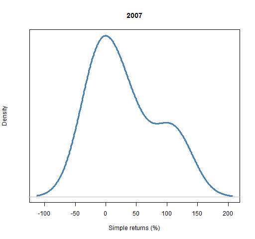
The result is that sretAnn07 is a vector of numbers that is as long as the number of random portfolios. We can plot the density of the returns with the simple command:
plot(density(sretAnn07))
But we can also make it prettier with a little effort (Figure 2).
Figure 2: Distribution of simple returns for 2007. 
The command to create Figure 2 is:
plot(density(sretAnn07 * 100), main="2007",
   xlab="Simple returns (%)", yaxt="n",
   col="steelblue", lwd=3)
The first thing we do is multiply the returns by 100 to put them into percent.
We give the main argument something useful (if you don’t want a main title, then say main="").
The use of yaxt in this way removes the unenlightening numbers along the y-axis.
The color of the density line is controlled by the col argument, and its width by lwd (the default is 1).
Explanation
The apply function allows you to apply a function to columns of a matrix (as here if the second argument is 2). When the second argument is 1, then the function is applied to the rows.
Hence we are getting the standard deviation of each column. To annualize the standard deviations we multiply by the square root of 252 (because there are about 252 trading days in a year), and then we multiply by 100 to get percent.
See also
Navigate
- Back to “Random Portfolio Generation”
- Back to the top level of “Portfolio Probe Cookbook”
