Task
Generate random portfolios with restrictions on volatility or tracking error.
Preparation
This presumes that you can do basic random portfolio generation. For example, that you have mastered “Very simple long-only”.
- Portfolio Probe
You need to have the Portfolio Probe package loaded into your R session:
require(PortfolioProbe)
If you don’t have Portfolio Probe, see “Demo or Buy”.
Doing the example
- The objects:
priceVector,grossVal,curPortfolthat are defined in several examples, such as in “Passive, no benchmark (minimum variance)” xaLWvar06variance matrix from “Returns to variance matrix” examplexaLWvar06EqWtvariance matrix from “Add benchmark to variance matrix” examplepprobeDatapackage
You need to have the package loaded into your R session:
require(pprobeData)
Doing it
We generate random portfolios with the following constraints:
- maximum volatility
- volatility within a range
- maximum tracking error
- tracking error within a range
maximum volatility
We generate 1000 random portfolios with volatility at most 12%:
rpVolMax <- random.portfolio(1000, priceVector,
   long.only=TRUE, gross=grossVal, variance=xaLWvar06,
   existing=curPortfol, var.constraint=.12^2/252)
We need to transform the 12% volatility into the scale of our variance matrix, which is daily.
volatility within a range
To impose a range on volatility, you need to give a two-column matrix as the var.constraint argument. Here we constrain the volatility to be between 11.9% and 12%:
rpVolRange <- random.portfolio(1000, priceVector,
   long.only=TRUE, gross=grossVal, variance=xaLWvar06,
   existing=curPortfol,
   var.constraint=rbind(c(.119, .12)^2/252))
The value given to var.constraint looks like:
> rbind(c(.119, .12)^2/252)
             [,1]         [,2]
[1,] 5.619444e-05 5.714286e-05
You could get the same thing with:
> t(as.matrix(c(.119, .12)^2/252))
             [,1]         [,2]
[1,] 5.619444e-05 5.714286e-05
maximum tracking error
Tracking error is constrained with the bench.constraint argument. But this argument is on the variance scale — that is, some scaling of the squared tracking error.
The variance we are using is from daily returns. We want 1000 portfolios that have at most 2% (predicted) tracking error.
rpTEmax <- random.portfolio(1000, priceVector,
   long.only=TRUE, gross=grossVal,
   variance=xaLWvar06EqWt, existing=curPortfol,
   bench.constraint=c(EqWt=.02^2/252))
There must be a name on the value given to bench.constraint so that it knows which asset to use as the benchmark.
tracking error within a range
We generate 1000 random portfolios with predicted tracking error that is between 3.5% and 4%:
rpTErange <- random.portfolio(1000, priceVector,
   long.only=TRUE, gross=grossVal,
   variance=xaLWvar06EqWt, existing=curPortfol,
   bench.constraint=rbind(EqWt=c(.035, .04)^2/252))
The value given to bench.constraint in this case is a matrix with one named row and two columns:
> rbind(EqWt=c(.035, .04)^2/252)
             [,1]         [,2]
EqWt 4.861111e-06 6.349206e-06
Explanation
The var.constraint argument constrains the variance. If it is given one number, then that is taken to be the maximum value allowed. To specify a range, you give a two-column matrix where the first column gives the minimum allowed, and the second column gives the maximum allowed. (A vector of values would be maximums for multiple variances.)
The bench.constraint argument takes values just like var.constraint except that the value or the row needs to be named with the identifier of the benchmark.
Further details
It is possible to constrain both volatility and tracking error. Here we constrain volatility to be between 11% and 12% and the tracking error to be 3.5% to 4%:
rpVolTErange <- random.portfolio(1000, priceVector,
   long.only=TRUE, gross=grossVal,
   variance=xaLWvar06EqWt, existing=curPortfol,
   bench.constraint=rbind(EqWt=c(.035, .04)^2/252),
   var.constraint=rbind(c(.11, .12)^2/252))
Remember that since we are using argument names, the order of the arguments doesn’t matter (except in this case the number of portfolios to generate and the prices).
Checking your work
predicted volatility
We can check that the volatility is really being restricted by collecting the ex-ante variances for the portfolios:
volCheck <- sqrt(252 * unlist(randport.eval(rpVolMax,
   keep='var.values')))
The volCheck object holds the predicted volatility for each portfolio. The randport.eval function gets the answer that the optimizer would have if it arrived at the random portfolio. You then have the option to keep only some components of the answer (or to apply a function to it). In this case we are keeping only the predicted variances.
We can look at the achieved volatilities:
> summary(volCheck)
   Min. 1st Qu.  Median    Mean 3rd Qu.    Max.
0.08973 0.11150 0.11610 0.11430 0.11880 0.12000
> tail(sort(volCheck))
var.values.V0 var.values.V0 var.values.V0
    0.1199847     0.1199902     0.1199902
var.values.V0 var.values.V0 var.values.V0
    0.1199926     0.1199931     0.1199993
This exercise would be slightly more complicated for the portfolios that constrain tracking error because in that case there are two values in the var.values component: the portfolio variance and the variance relative to the benchmark.
realized volatility
We can use the moves in “Returns and realized volatility” to get the realized volatility for the subsequent year and then plot the distribution.
retVolMax07 <- valuation(rpVolMax,
   xassetPrices[251:502,], returns="log")
volVolMax07 <- apply(retVolMax07, 2, sd) *
   sqrt(252) * 100
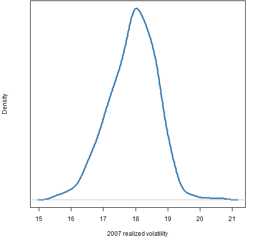
plot(density(volVolMax07)) # essentially Figure 1
Figure 1: Volatility realized in 2007 for the rpVolMax portfolios. 
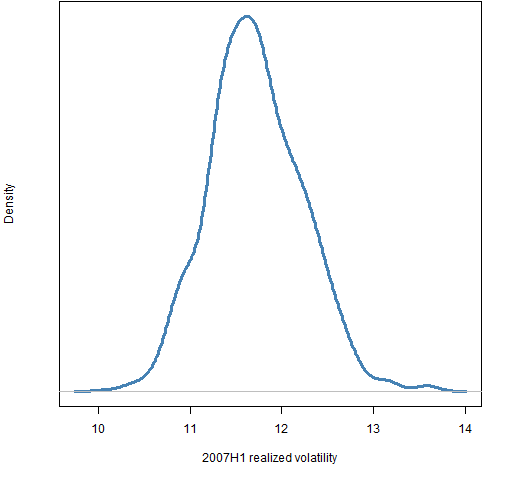
The realized volatility for all of the portfolios is significantly bigger than 12%. However, that need not mean we have done anything wrong because 2007 is when volatility started to heat up. We can look at the realized volatility in the first half of 2007 when volatility was still low.
retVolMax07H1 <- valuation(rpVolMax,
   xassetPrices[251:376,], returns="log")
volVolMax07H1 <- apply(retVolMax07H1, 2, sd) *
   sqrt(252) * 100
Figure 2: Volatility realized in H1 of 2007 for the rpVolMax portfolios.  This is a more reassuring picture.
Troubleshooting
- Are you giving
var.constraintorbench.constrainta value (or values) that correspond to the variance matrix that you are using? Is the variance for returns or percent returns? What is the time frame of the returns?
- If you are wanting a range for the volatility or tracking error, are you giving a two-column matrix?
See also
Navigate
- Back to “Random Portfolio Generation”
- Back to the top level of “Portfolio Probe Cookbook”
