Historical Value at Risk (VaR) is very popular because it is easy and intuitive: use the empirical distribution of some specific number of past returns for the portfolio.

Previously

“The estimation of Value at Risk and Expected Shortfall” included an R function to estimate historical VaR.

Generating portfolios

A useful tool to explore risk models is random portfolios.  Generate a number of portfolios that look like portfolios you might actually hold, and then see how well the risk model performs on these portfolios.

In this case 1000 long-only random portfolios were generated with exactly 60 stocks that had a maximum weight of 4% at the point when the portfolios were created (the end of 2006).  The universe was almost all of the constituents of the S&P 500 at a particular point in time.

Daily historical VaR using 500 days was estimated for each available time.  The time period over which we have VaR estimates is the start of 2008 to a few days into 2012.

VaR exceedences

We have VaR estimates for the 1000 portfolios on each of 1047 days.  The VaR values are for a 5% probability.  That is, we expect the actual loss to exceed the VaR about 5% of the time.

A hit happens when the VaR is exceeded.

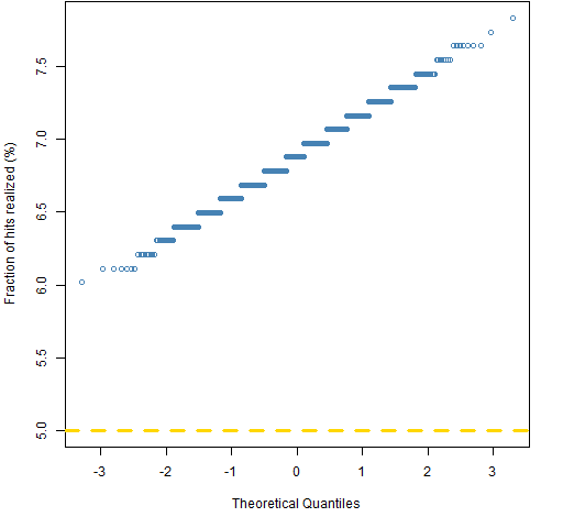
Figure 1 shows the fraction of hits that occurred for each portfolio.

Figure 1: Normal QQplot of the fraction of hits for 1000 random portfolios. This shows that the hit rate was substantially higher than 5% for all of the portfolios.  That all of the portfolios are so far above the desired value is a hint that they are going to be statistically significantly higher.

Because of how historical VaR is created, it must have the right average level in the long run.  However, it can be quite different in the short run.

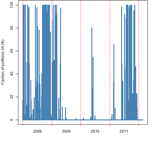
These two points suggest that there can be clustering of hits through time.  Figure 2 shows another view of the same hit data.

Figure 2: Fraction of portfolios that are hit on each day. You may be concerned that there are days on which all the portfolios are hit.  That’s not a problem.  Some days almost all the assets go up, there are likely to be no hits on those days.  Some days almost all the assets go down, there are likely to be lots of hits on those days.

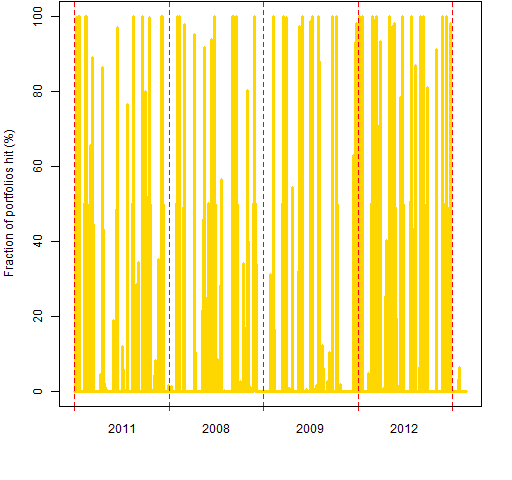
What is not right about Figure 2 is that there are long periods of lots of hits and long periods of pretty much no hits.  Figure 3 gives us a sense of what such plots should look like by randomly permuting the values that are plotted in Figure 2.

Figure 3: Randomly permuted fraction of portfolios that are hit on each day. That the years shown in Figure 3 are random was accidental, but useful in emphasizing that this is fantasy and not reality.

Summary

Volatility clustering causes historical VaR to have periods of lots of hits followed by periods of very few hits.  There is a price to be paid for its simplicity and intuitiveness.

Appendix R

generate random portfolios

The Portfolio Probe software is required to generate the portfolios:

require(PortfolioProbe)

rp60port <- random.portfolio(1000, sp5.close[250,], 
   gross=1e6, long.only=TRUE, max.weight=.04, 
   port.size=c(60,60))

The random portfolio command generates 1000 portfolios using row 250 of the closing price matrix as the asset prices.  The gross value is set to be $1 million (we don’t really care what value the portfolios have).  The portfolios are constrained to be long-only, the maximum weight of all assets is set to 4%, and the number of assets in the portfolio is set to be exactly 60.

portfolio returns

Portfolio Probe includes a function that will produce a matrix of returns of the random portfolios:

rp60ret <- valuation(rp60port, sp5.close, 
   returns="log")

VaR estimation

Here we first create an object to hold the VaR estimates for the random portfolios, and then fill it with the estimates:

rp60hist500VaR <- rp60ret
rp60hist500VaR[] <- NA
vseq <- -500:-1
for(i in 501:1547) {
  tseq <- vseq + i
  for(j in 1:1000) {
    rp60hist500VaR[i,j] <- VaRhistorical(rp60ret[tseq,j],
        digits=15)
  }
}

“The estimation of Value at Risk and Expected Shortfall” gives the definition of VaRhistorical.

VaR hits

We use the portfolio returns and the VaR estimates to get the hits:

rp60hist500hit <- rp60ret < -rp60hist500VaR

The values in the hit matrix are TRUE when the loss exceeded the VaR and FALSE otherwise.

spaces in R

Almost all the time it doesn’t matter — except for readability — if you put spaces into R commands.  But lets look at the command above without spaces:

rp60hist500hit<-rp60ret<-rp60hist500VaR

The result of this command would be different.  We would end up with three objects that contained the VaR estimates.

This is Circle 8.1.30 of The R Inferno.

time plots

Figures 2 and 3 depend on pp.timeplot which you can put into your R session with:

source('https://www.portfolioprobe.com/R/blog/pp.timeplot.R')