What is variance targeting in garch estimation?  And what is its effect?

Previously

Related posts are:

• A practical introduction to garch modeling
• Variability of garch estimates
• garch estimation on impossibly long series

The last two of these show the variability of garch estimates on simulated series where we know the right answer.  In response to those, Andreas Steiner wondered about the effect of variance targeting on the results.

Concept

Maximization of garch likelihoods turns out to be a surprisingly nasty optimization problem.  It used to be that computers were slower and the algorithms used to optimize garch were less sophisticated.  The idea of variance targeting was born in that environment.

In a garch(1,1) model if you know alpha, beta and the asymptotic variance (the value of the prediction at infinite horizon), then omega (the variance intercept) is determined.  Variance targeting is the act of specifying the asymptotic variance in order not to have to estimate omega.

The assumed asymptotic variance could be anything, but the exceedingly most popular choice is the unconditional variance of the series.

The usual result of using variance targeting is that the optimization is quicker, and (for some optimizers) more likely to be near the global optimum.

Experiment

Series were generated from a garch(1,1) model using t-distributed errors with 7 degrees of freedom.  The previous posts did this without variance targeting for series of lengths 2000 and 100,000.  The same thing was done with variance targeting (using different generated series).  Each run consisted of 1000 series.

Estimate distributions

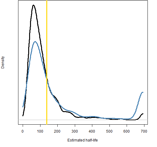
Figures 1 and 2 compare the half-life estimates with and without variance targeting.  The vertical gold line in the distribution plots shows the true value.

Figure 1: Distribution of half-life estimates with 100,000 observations; variance targeting (black), no targeting (blue). 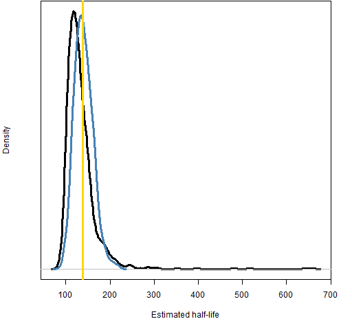Figure 2: Distribution of half-life estimates with 2000 observations; variance targeting (black), no targeting (blue). Figures 3 and 4 compare the estimated asymptotic variance with and without variance targeting.  This is a simple estimation with variance targeting and a derived estimate without it.

Figure 3: Distribution of asymptotic variance estimates with 100,000 observations; variance targeting (black), no targeting (blue).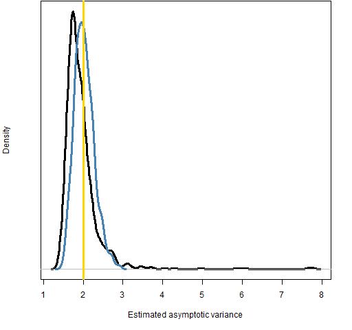

Figure 4: Distribution of asymptotic variance estimates with 2000 observations; variance targeting (black), no targeting (blue). 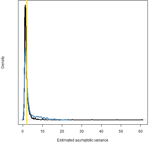Figures 5 and 6 compare the degrees of freedom estimates.

Figure 5: Distribution of degrees of freedom estimates with 100,000 observations; variance targeting (black), no targeting (blue).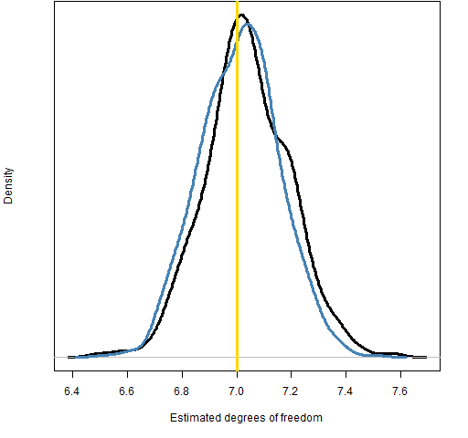

Figure 6: Distribution of degrees of freedom estimates with 2000 observations; variance targeting (black), no targeting (blue).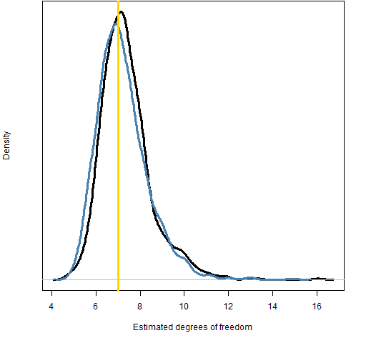

Figures 7 and 8 compare the alpha estimates.

Figure 7: Distribution of alpha estimates with 100,000 observations; variance targeting (black), no targeting (blue).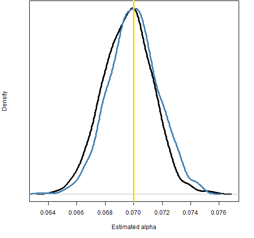

Figure 8: Distribution of alpha estimates with 2000 observations; variance targeting (black), no targeting (blue).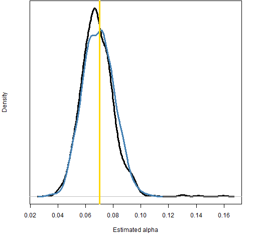

Figures 9 and 10 compare the beta estimates.

Figure 9: Distribution of beta estimates with 100,000 observations; variance targeting (black), no targeting (blue).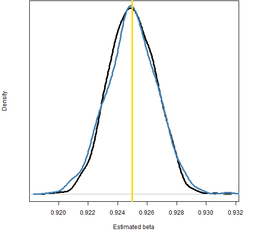

Figure 10: Distribution of beta estimates with 2000 observations; variance targeting (black), no targeting (blue).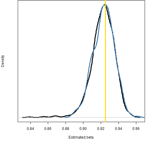

Figures 11 and 12 compare the estimates of omega.

Figure 11: Distribution of omega estimates with 100,000 observations; variance targeting (black), no targeting (blue).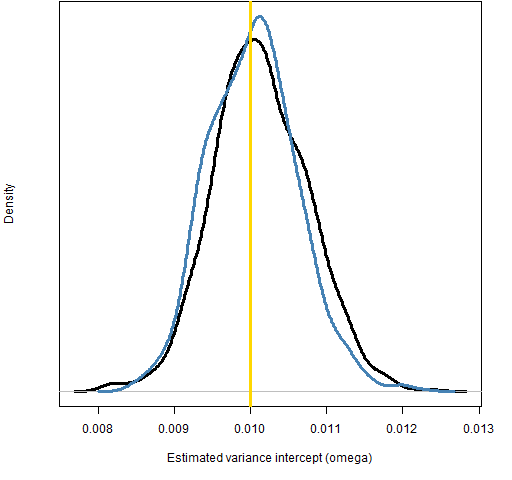

Figure 12: Distribution of omega estimates with 2000 observations; variance targeting (black), no targeting (blue).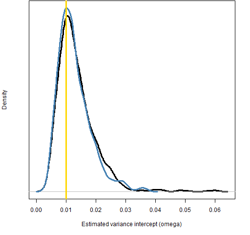

Mean squared error

We can boil down the distributions into one number: the mean of the squared difference between the estimate and the true value.  Mean squared error should not be thought of as the magic bullet, but it is sometimes useful.  I think this is a case where it is useful.

Figure 13 shows the ratios of  mean squared errors (MSE for variance targeting divided by MSE without targeting) for the parameters that are directly estimated.

Figure 13: Ratio of mean squared errors for estimated parameters between variance targeting and not; bigger than 1 means that variance targeting is worse. 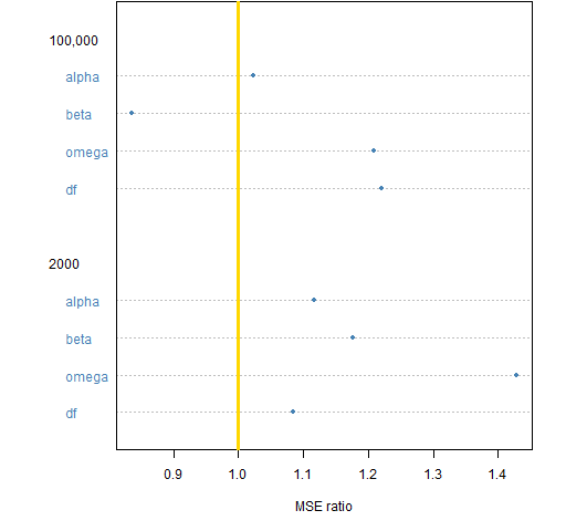We see that variance targeting tends to be slightly bad for the mean squared error of the estimated parameters.

Figure 14 shows the mean squared error ratios for the derived quantities — what we are actually more interested in.

Figure 14: Ratio of mean squared errors for derived quantities between variance targeting and not; bigger than 1 means that variance targeting is worse. 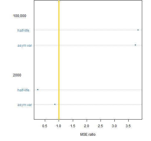There is an interesting pattern for these values.  Variance targeting provides a substantial improvement when there are 2000 observations, but is quite detrimental when there are 100,000 observations.

For a “small” number of observations (2000), variance targeting is worse for the individual parameters but better for useful quantities.  It wins the war after losing every battle.

I suspect that the best way to think about this is with Bayesian statistics.  Variance targeting imposes the prior that the asymptotic variance is equal to the unconditional variance of the series.  This is an informative restriction when there are not many observations.  But as the number of observations grows, the restriction drags us away from the right value rather than dragging us towards it.

Compute time

The time to do the computations was reduced with variance targeting.  For series of 2000 the variance targeting took about 72% of the computer time of the estimation without targeting.  For series of 100,000 the figure is 79%.

Summary

This experiment suggests that variance targeting is a useful tool — not because it speeds computation (although it does) — but because the estimate (for realistic series lengths) tends to have better properties.

Epilogue

They say I shot a man named Gray, and took his wife to Italy.
She inherited a million bucks, and when she died it came to me.
I can’t help it if I’m lucky.

from “Idiot Wind” by Bob Dylan

Appendix R

Here is how this was done in R.

estimation

The estimation was done with the rugarch package.  The specification with variance targeting is:

require(rugarch)
tvtspec <- ugarchspec(mean.model=list(armaOrder=c(0,0)),
   distribution="std",
   variance.model=list(variance.targeting=TRUE))

More details about the estimation are shown in “Variability of garch estimates”.

mean squared errors

The function that was written to compute the mean squared errors was:

pp.garmse <- function(first, second, 
    parameters=c(.01, .07, .925, 7))
{
  # placed in public domain 2012 by Burns Statistics

  # test status: not tested

  ans <- array(NA, c(6,3), list(c('alpha', 'beta', 'omega', 
     'df', 'avar', 'halflife'), c('first', 'second', 'ratio')))
  ans['alpha', 'first'] <- mean((first[,'alpha1'] - parameters[2])^2)
  ans['alpha', 'second'] <- mean((second[,'alpha1'] - parameters[2])^2)
  ans['beta', 'first'] <- mean((first[,'beta1'] - parameters[3])^2)
  ans['beta', 'second'] <- mean((second[,'beta1'] - parameters[3])^2)
  ans['omega', 'first'] <- mean((first[,'omega'] - parameters[1])^2)
  ans['omega', 'second'] <- mean((second[,'omega'] - parameters[1])^2)
  ans['df', 'first'] <- mean((first[,'shape'] - parameters[4])^2)
  ans['df', 'second'] <- mean((second[,'shape'] - parameters[4])^2)
  avar <- parameters[1] / (1 - sum(parameters[2:3]))
  hl <- log(.5) / log(sum(parameters[2:3]))
  av.f <- first[,'omega'] / (1 - first[,'alpha1'] - first[,'beta1'])
  hl.f <- log(.5) / log(first[,'alpha1'] + first[,'beta1'])
  av.s <- second[,'omega'] / (1 - second[,'alpha1'] - second[,'beta1'])
  hl.s <- log(.5) / log(second[,'alpha1'] + second[,'beta1'])
  ans['avar', 'first'] <- mean((av.f - avar)^2)
  ans['avar', 'second'] <- mean((av.s - avar)^2)
  ans['halflife', 'first'] <- mean((hl.f - hl)^2)
  ans['halflife', 'second'] <- mean((hl.s - hl)^2)
  ans[,'ratio'] <- ans[,'second'] / ans[,'first']
  attr(ans, "call") <- match.call()
  ans
}

This function was used like:

gmse.100K.07 <- pp.garmse(ges.a.100K.07, ges.vt.100K.07)
gmse.2000.07 <- pp.garmse(ges.a.2000.07, ges.vt.2000.07)

dotchart

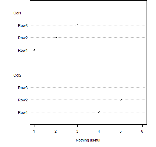
Dotcharts are a visually efficient way of presenting data that is often presented with barplots.  Here is a small example similar to Figures 13 and 14.

First we create a matrix to use in the example:

dmat <- array(1:6, c(3,2), list(paste0("Row", 1:3), 
   paste0("Col", 1:2)))

(The paste0 function is a recent addition, you can do the same thing using paste with sep="".)

Our matrix looks like:

> dmat
     Col1 Col2
Row1    1    4
Row2    2    5
Row3    3    6

The command that creates Figure 15 is:

dotchart(dmat, xlab="Nothing useful")

Figure 15: Example dotchart.