Does minimum variance act differently from low volatility?  Do either of them act like low beta?  What about high volatility versus high beta?

Inspiration

Falkenblog had a post investigating differences in results when using different strategies for low volatility investing.  Here we look not at a single portfolio of a given strategy over time, but a thousand.

Ingredients

The data are daily closing prices of almost all of the stocks in the S&P 500.  The final date in the data is 2012 February 24.

The in-sample period was 2006.  That is the period in which the variance matrix — and hence the volatilities — were estimated.  The betas relative to the S&P 500 were also estimated using 2006 data.

Figure 1: The volatility versus beta estimates from 2006. 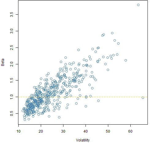Figure 1 demonstrates that the belief that beta is about volatilty really is a myth.  Note that the stock with the largest volatility (RHT) has a beta of 0.97.

The portfolios were formed as of the start of 2007.

Constraints

All the portfolios were built with these three constraints:

1. long-only
2. 45 to 50 names in the portfolio
3. all assets have (starting) weights of no more than 4%

Six sets of random portfolios (1000 in each set) were generated.  The additional constraints were:

• vanilla: (no additional constraints)

• low variance: the portfolio variance is no more than 120% of the minimum attainable variance (as estimated from 2006) given the first three constraints

• low volatility: only stocks from the lowest quartile of volatilities (as estimated from 2006)

• low beta: only stocks from the lowest quartile of betas (as estimated from 2006)

• high volatility: only stocks from the highest quartile of volatilities (as estimated from 2006)

• high beta: only stocks from the highest quartile of betas (as estimated from 2006)

Results over time

Figures 2 through 7 show the valuations over time of the random portfolios (in blue).  These are buy-and-hold portfolios — there is no trading.

The black line shows the median valuation at each point in time.  The gold lines delimit the central 95% of valuations at each timepoint.  None of these three lines follows a particular portfolio.

Figure 2: The “vanilla” portfolio values.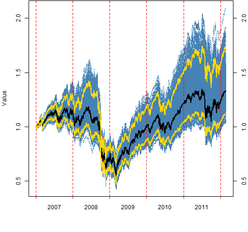

Figure 3: The “low variance” portfolio values.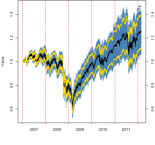

Figure 4: The “low volatility” portfolio values.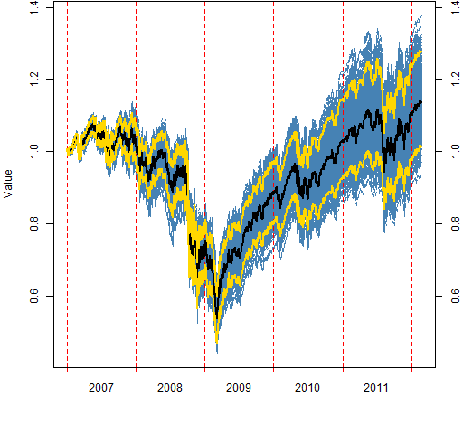

Figure 5: The “low beta” portfolio values.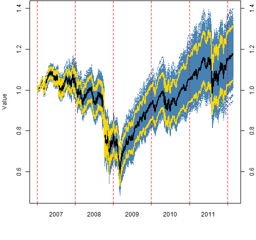

Figure 6: The “high volatility” portfolio values.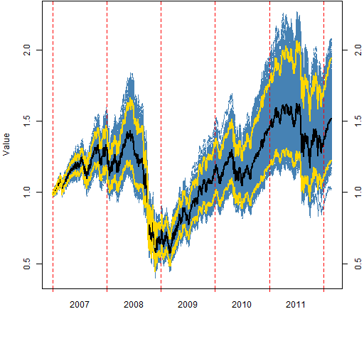

Figure 7: The “high beta” portfolio values.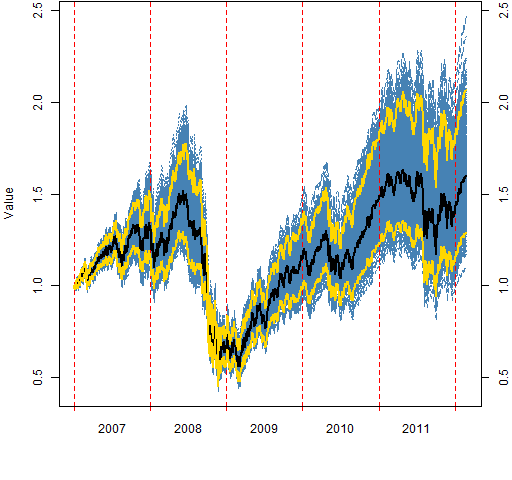

Caveat

These results have significant survival bias.

This is not selecting S&P 500 stocks in 2007.

This is selecting stocks in 2007 that will be in the S&P 500 in 2012.

Summary

Not forgetting the caveat above, what I see is:

• low volatility and low beta look quite similar
• low variance performed better during the period than either low volatility or low beta
• there are subtle — and perhaps superficial — differences between high volatility and high beta
• the vanilla (and high vol and beta) portfolios have an extraordinary spread in valuation by mid-2008; the spread then seriously collapses (Why?)
• In contrast 2011 August looks more like a fault line in geological strata

Update — posts that go farther with these data are:

• “Beta is not volatility”
• “Rebalancing the low vol cohorts”
• “Maximum weight of the low vol cohorts”
• “Betas of the low vol cohorts”

Appendix R

estimate betas

Estimating the betas is one line of R code:

sp5.beta06 <- coef(lm(sp5.ret[1:250,] ~ spxret[rownames(sp5.ret)[1:250]]))[2,]

generate random portfolios

require(PortfolioProbe)

Select the subset of stock ids that are desired:

bp03.betaq1 <- names(sp5.beta06)[sp5.beta06 < quantile(sp5.beta06, .25)]

Now use that in specifying the portfolios to create:

bpo3.rp.lowbeta <- random.portfolio(1000, prices=sp5.close[251,], gross=1e6, long.only=TRUE, port.size=c(45, 50), max.weight=.04, universe=bp03.betaq1)

valuation

It is just one command to get the matrix of valuations over time for each set of random portfolios:

bp03.rpval.lowbeta <- valuation(bp03.rp.lowbeta, sp5.close[-1:-250,], collapse=TRUE)

plot

The function used to do the plotting (x is the valuation matrix) is:

> pp.valplot
function (x, scale=1e6, ...)
{
        x <- x / scale
        pp.timeplot(x, ylab="Value", div="years",
               col="steelblue", ...)
        med <- apply(x, 1, median)
        ci <- apply(x, 1, function(y)
                quantile(y, c(.025, .975)))
        lines(med, col="black", lwd=2)
        matlines(t(ci), col="gold", lwd=2, lty=1)
        axis(4)
}

This uses the pp.timeplot function.

Subscribe to the Portfolio Probe blog by Email