The return of a hypothetical fund was 17.9% in 2010.  We want to know if that is good or bad.

The benchmark method

The assets in the portfolio are constituents of the S&P 500, so we can compare our fund return to the return of the index.

Figure 1: 2010 returns of: the fund and the S&P 500. 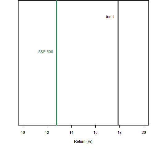That looks pretty good for the fund.  But is it?

One problem is that our fund may have characteristics that are not much like the index.  But even if we had the perfect benchmark, there is still a problem.  We don’t know if the difference in returns between our fund and the benchmark is big or small — was it skill or luck?  Our fall-back position is to test the difference over multiple periods, but it will take decades of data to know anything that way.

And, as we’ll see, we’re being a bit naive here all together.

The peer group method

Figure 2: 2010 returns of the fund and the distribution of the returns of “peers”. 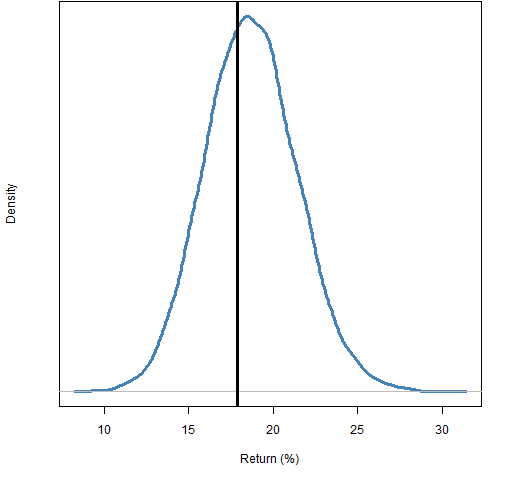 Now the fund appears not to be special at all.

We can imagine that the distribution in Figure 2 is the distribution of the returns of the peers of our fund.  This is a common approach, but it really doesn’t get us far.  We know where our fund is in the distribution but we don’t know what that means.  We don’t know how much of that distribution is skill and how much is luck.  Peer groups are used as if it were all skill.  However, it is probably mostly luck.

In actuality Figure 2 is not the distribution of peers — it is the distribution of returns of random portfolios that have the same constraints as the fund.  In this case we know how much of the distribution is skill and how much is luck.  It is all luck.

Now we actually know something about the performance of our fund.

But, as we’ll see, we know less than we think we do.

Decisions

What do we really want to measure when doing performance measurement?  I claim we want to measure the effect of decisions.

Lumping all decisions together isn’t especially helpful.  One way to divide the decisions for the fund is:

• those made before the start of 2010
• those made during 2010

We can get the “luck distribution” of the 2010 decisions by mimicking them with random trades.  We trade away from the portfolio as it was at the start of the year, obeying the portfolio and turnover constraints of the fund, but otherwise moving randomly.  We get the distribution of the 2010 returns based on the decisions the fund manager might have made during 2010.  This is the gold distribution in Figure 3.

Figure 3: 2010 returns of: the fund (black line), fund at start of 2010 (gold line), distribution of static portfolios (blue), and distribution of 2010 decisions (gold). 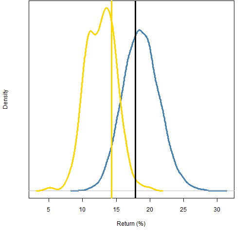The gold line shows the return the portfolio would have had during 2010 if there had been no trading in the fund.  (The gold line is logically at the center of the gold distribution, but we can see that it need not really be at the center.  If the gold line were at the worst possible portfolio for the period, the gold distribution would be mostly above it.)

Now we really can say something about the decisions:

• The decisions made in 2010 were good for returns in 2010 (black line compared to gold distribution).
• The decisions made prior to 2010 were bad for returns in 2010 (gold line compared to blue distribution).

Another way of looking at it is that we are dividing the portfolio into a static part and a dynamic part.  We compare the static part of the portfolio to static random portfolios, and we compare the dynamic part to dynamic random portfolios.

Short-termism

You may be concerned that this is just encouraging short-term performance. We get very good information on how the decisions affect immediate returns.

That’s an excellent concern.

But the decision period and the evaluation period need not coincide.  Figure 4 inspects the quality of the 2010 decisions for returns in the first half of 2011.

Figure 4: 2011H1 returns of: the fund at end of 2010 (black line), fund at start of 2010 (gold line), distribution of static portfolios (blue), and distribution of 2010 decisions (gold). 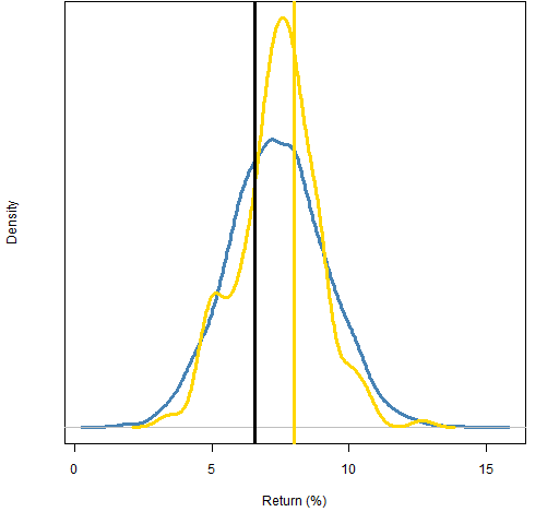What we learn from Figure 4:

• The decisions made in 2010 were a slight disadvantage during 2011H1 (black line compared to gold distribution).
• The decisions made prior to 2010 were essentially neutral in 2011H1 (gold line compared to blue distribution).
• The decisions made prior to 2011 were essentially neutral in 2011H1 (black line compared to blue distribution).
• The trading done during 2010 is — at the midpoint of 2011 — ahead of doing no trading by a return of about 2%.  The traded portfolio lost ground to the no-trade portfolio during 2011H1, but is ahead over all.

Note that the black line in Figure 4 is not representing (exactly) the same thing as the black line in Figure 3.  The black line in Figure 3 is for the dynamic fund as it changed throughout 2010, but in Figure 4 it is static — the final portfolio of the period.  The same applies to the gold distributions.

Summary

• investment performance measurement is about decisions
• the decision period and the evaluation period need not — and often should not — be the same: decisions can be evaluated years after they are made
• random portfolios allow us to gauge luck versus skill
• static portfolios should be compared to static random portfolios, and dynamic portfolios should be compared to dynamic random portfolios

Appendix R

The main computations are just like those described in chapter 5 of the Portfolio Probe User’s Manual.

Extending to different time frames is trivial.  A new set of static portfolios needs to be generated using prices at the new starting time:

require(PortfolioProbe)

rpstatic11 <- random.portfolio(1e4, prices=sp500.price1011[253,], max.weight=.05, sum.weight=c('10'=.3), long.only=TRUE, gross=1e6)

The constraints here are long-only, no asset weight greater than 5%, the sum of the 10 largest asset weights no larger than 30% and the gross value of the portfolio very close to 1 million dollars.

Once that is done, we have two sets of static distributions and two static portfolios for which we need to compute returns over the new time period.  That can be done with commands like:

rpstatic11.ret <- pp.simpret(valuation(rpstatic11, prices=sp500.price1011[c(253,378),], collapse=TRUE))

Subscribe to the Portfolio Probe blog by Email