The S&P 500 returned 29.6% in 2013.  How might that have varied?

S&P weights

There are many features that could vary — here we will keep the same constituents (almost) and weights with similar sizes but that are randomly assigned rather than based on market capitalization.

That is, we want the large weights of our hypothetical indices to have similar sizes as the actual weights in the S&P.  Figure 1 shows the cumulative sum of the 10 largest weights as listed on slickcharts.

Figure 1: Cumulative sum of the largest weights in the S&P 500.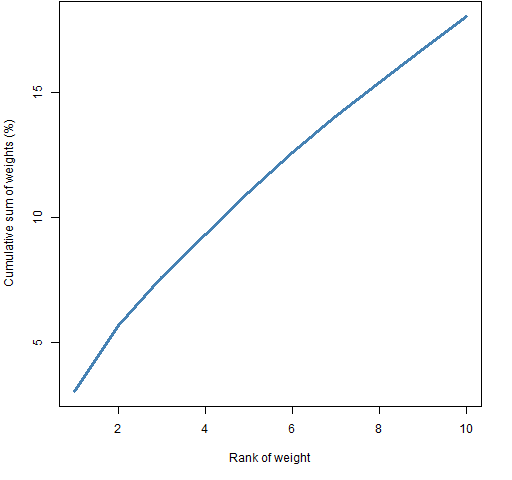 

The largest weight is listed as 3.04% for Apple.  The sum of the 5 largest weights is 11.03% and the sum of the 10 largest is 18.06%.

Might have been

Figure 2 shows the distribution of the 2013 returns for random portfolios that have their largest weight slightly more than 3%, the sum of their 5 largest weights slightly more than 11% and the sum of their 10 largest weights slightly more than 18%.

Figure 2: Distribution of 2013 returns for random portfolios with largest weight constraints similar to the S&P 500 weights.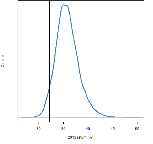 

As is suggested by the analysis (just below) of the largest stocks, it seems that the total return of SPY of about 32.2% is a more realistic reference than 29.6%

The stars above

If we look at the top 10 stocks on their own, then the largest weight among them is about 17% and the smallest weight is about 7%.  Figure 3 shows the distribution of returns from random portfolios of the 10 largest stocks where their weights range from 20% to 7%.

Figure 3: Distribution of 2013 returns of portfolios of the 10 largest stocks; the vertical line shows the return of the portfolio of the 10 stocks with weights in the same ratio as the S&P weights.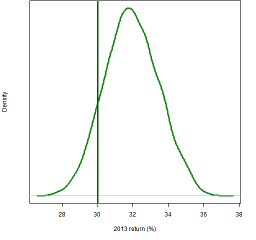 

Figure 4 compares the distributions in Figures 2 and 3.

Figure 4: Distribution of the 2013 returns of the portfolios with all stocks (blue) and the portfolios of the 10 largest stocks (green).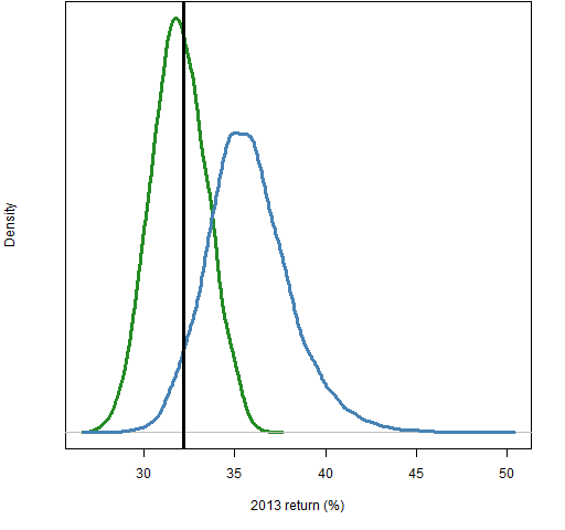 

Clearly the large stocks didn’t perform as well as the typical stock in the S&P 500.

Decreasing the largest weights

Here we return to portfolios containing all of the stocks.

Figure 5 gives some hint of the effect of the size of the largest weights.  The gold distribution is for random portfolios where the sum of weights constraints are halved.  That is, the largest weight is slightly more than 1.5%, the sum of the 5 largest weights is slightly more than 5.5% and the sum of the 10 largest weights is slightly more than 9%.

Figure 5: Distributions of 2013 returns of random portfolios with weight constraints like the S&P (blue) and those constraints halved (gold).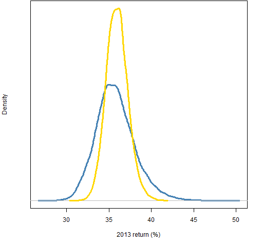 

The standard deviation of the returns of the portfolios with halved weight constraints is slightly bigger than half the standard deviation from the portfolios with the S&P-like constraints.

Summary

It’s easy for us to take an index too seriously — an index is just one particular trading strategy.  We should try to free ourselves.

Epilogue

I’m through with a-countin’ the stars above
And here’s the reason that I’m so free

from “Bye Bye Love” by Felice and Boudleaux Bryant

Appendix R

Computations and graphs were done in R.

weights plot

The largest weights are:

bigWeights <- c(3.04, 2.66, 1.91, 1.72, 1.70, 
   1.57, 1.46, 1.34, 1.34, 1.32)

A simple version of Figure 1 is:

plot(cumsum(bigWeights), type="l")

The data that are plotted are the cumulative sums of the largest 10 weights.  The type of plot is line.

The actual command that created Figure 1 is:

plot(cumsum(bigWeights), type="l", lwd=3, 
   col="steelblue", xlab="Rank of weight", 
   ylab="Cumulative sum of weights (%)")

constraints matrix

The specification of the limits for the sums of largest weights requires a matrix that has the minimum bound in the first column, the maximum bound in the second column, a row for each number of weights in the sum, and row names that are the number of weights in the sum.

An easy way to create such a matrix is to bind rows together:

conSumWt <- rbind("1"=c(.03, .031),
                  "5"=c(.11, .111),
                  "10"=c(.18, .181))

Note that these row names need to be quoted so that it is clear that they are meant to be row names.  If the row names are more typical names rather than numbers, then quotes are not necessary:

> rbind(a=c(2, 6), b=c(7, 9))
  [,1] [,2]
a    2    6
b    7    9

generate random portfolios

The Portfolio Probe software is necessary to generate the random portfolios:

require(PortfolioProbe)
nStocks <- ncol(univclose17)
rp13.sw1 <- random.portfolio(1e4, 
   prices=univclose17[1,], gross=1e9,
   long.only=TRUE, sum.weight=conSumWt,
   min.weight.thresh=.0002,
   port.size=c(nStocks, nStocks))

This last command generates 10,000 random portfolios using the prices on the close of the last day in 2012 for the 481 stocks from the S&P 500 that survived the year with full data.  The gross value is set to one billion dollars — the actual value is immaterial as long as it is large enough that the smallest weights imply positions substantially bigger than the prices.

The portfolios are constrained to be long-only, to have the sums of largest weights constrained as already discussed, and for all stocks to be in the portfolio with a weight of at least 2 basis points.

The alternative set of random portfolios is generated precisely the same except for the constraint:

sum.weight=conSumWt/2

random portfolios of the 10 largest stocks

The identifiers for the largest stocks are:

bigTicks <- c('AAPL', 'XOM', 'GOOG', 'MSFT', 'GE',
   'JNJ', 'CVX', 'PG', 'JPM', 'WFC')

The random portfolios are generated like:

rp13.big1 <- random.portfolio(1e4, 
   prices=univclose17[1,bigTicks], gross=1e9,
   long.only=TRUE, max.weight=.2,
   min.weight.thresh=.07, port.size=c(10, 10))

returns of random portfolios

The simple returns of the first set of portfolios is computed with:

rp13.sw1.ret <- valuation(rp13.sw1, 
   prices=univclose17[c(1,253),],
   returns="simple")