How does Value at Risk change through time for the same portfolio?

Previously

There has been a number of posts on Value at Risk, including a basic introduction to Value at Risk and Expected Shortfall.

The components garch model was also described.

Issue

The historical method for Value at Risk is by far the most commonly used in practice even though it has pretty much the worst statistical properties.

One reason it is popular is because it doesn’t move around very much from day to day for the same portfolio.  That property is what is explored here.

Another reason for the popularity of the historical method is that it is easy to understand.  You don’t need to know anything about exponential smoothing nor understand garch.

Example

A long history of the returns of the S&P 500 is used to get three 95% 1-day VaR estimates:

• 500-day historical
• normal distribution standard deviation estimated with exponential smooth (lambda=0.97)
• normal distribution standard deviation estimated with a components garch model assuming a t distribution

The normal distribution is used because of the irony that that is a conservative assumption in this case.

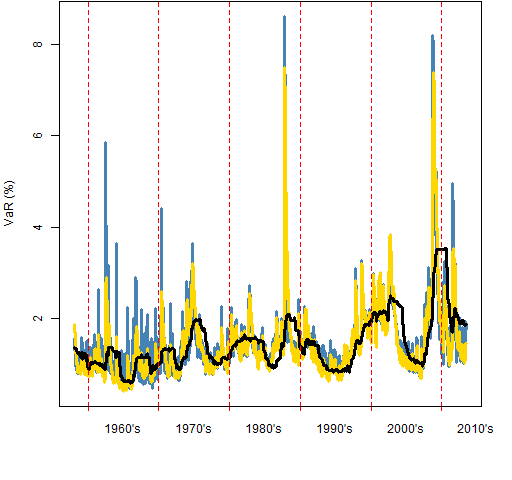
Figure 1 shows the three VaR estimates over the sample period.  The garch method has the highest highs, particularly in the 1960’s.  The historical method is dramatically smoother than the other two.

Figure 1: Value at Risk estimates for the S&P 500: garch prediction (blue), exponential smooth (gold), 2-year historical (black). 

Statistical tests

Two of the statistical tests for the quality of a Value at Risk estimate are:

• the binomial test to see if the fraction of hits (breaches) matches the probability level
• the Ljung-Box test to see if the timing of hits is predictable

Table 1 shows these tests of the quality of the Value at Risk estimates.  Since a 95% probability level is used, we want the percent of hits to be 5%.  The binomial p-value gives the probability of the percent of hits being farther from 5% than what is observed assuming that the true hit probability is 5%.  Small values mean it is not so easy to believe that the true value really is 5%.

The Ljung-Box test asks if the hits are predictable through time (specifically, if they are autocorrelated). Bigger numbers of the Ljung-Box statistic suggests more predictability.  For the lag 10 test performed, we start to get suspicious if the statistic is more than about 20.

Table 1: Binomial tests and Ljung-Box tests of the three estimates.

Estimator	Percent hits	Binomial p-value	Ljung-Box 10 statistic
garch	4.82	.352	51
exponential	5.40	.033	203
historical	5.54	.004	755

The garch estimate is substantially better than the others but still fails the  Ljung-Box tests.  The p-values for the Ljung-Box test are not shown because they are all very small.

Smoothness

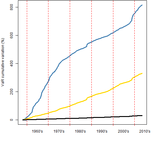
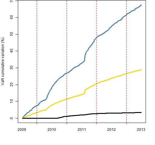
Figure 2 shows the differences in smoothness.  What is computed is the cumulative sum of the absolute differences from day to day.  Figure 3 shows the same thing for the final 1000 days.  Figure 2 suggests that the garch estimate is much more changeable in the 60’s and into the early 70’s than it is afterwards.

Figure 2: Cumulative sum of absolute daily differences of VaR estimates: garch prediction (blue), exponential smooth (gold), 2-year historical (black). 

Figure 3: Cumulative sum of absolute daily differences of VaR estimates of the final 1000 days: garch prediction (blue), exponential smooth (gold), 2-year historical (black). 

The final value for the historical method in Figure 3 is 3.4% as opposed to 29% for exponential smoothing and 67% for garch.  Presumably the true Value at Risk is even more variable than the garch estimate.

Summary

The historical method for Value at Risk is dramatically smoother than the reality.  Sometimes the sacrifice of statistical rigor is worth the extra smoothness.

Sacrificing so much rigor probably means we are asking the wrong question.

Epilogue

Comes a rainstorm, put your rubbers on your feet
Comes a snowstorm, you can get a little heat

from “Comes Love” by Lew Brown, Sam Stept and Charles Tobias

Appendix R

Computations were done with R.

update data

The series of returns was updated to the present.  The first thing was to get new levels back past where the existing data ended:

require(TTR)
spxnew2 <- getYahooData('^GSPC', 20130311, 20130628)
spxnewret2 <- diff(log(drop(as.matrix(spxnew2[, 
   "Close"]))))

Next is to look to see that the overlap matches:

tail(spxret)
head(spxnewret2)

Finally the two are spliced together:

spxret <- c(spxret, spxnewret2[-1:-3])

create objects

We are going to end up with three vectors of VaR estimates.  Here we create them, and will later fill them in.

spxVaRhist <- spxret
spxVaRhist[] <- NA
spxVaRexpsmo <- spxVaRgar <- spxVaRhist

estimate historical and exponential smooth

The historical and exponential smooth estimates are done in the same loop:

rseq <- -500:-1
for(i in 2001:length(spxret)) {
   tret <- spxret[rseq + i]
   spxVaRhist[i] <- VaRhistorical(tret, 
      prob=.05, digits=15)
   spxVaRexpsmo[i] <- VaRnormalExpsmo(tret,
      prob=.05, lambda=.97, digits=15)
}

estimate garch

require(rugarch)
comtspec <- ugarchspec(mean.model=list(
   armaOrder=c(0,0)), distribution="std",
   variance.model=list(model="csGARCH"))

gseq <- -2000:-1
spxgarsigma <- spxVaRgar
for(i in 5993:length(spxret)) {
   tgar <- try(ugarchfit(spec=tspec, spxret[gseq + i]))
   if(!inherits(tgar, "try-error")) {
      spxgarsigma[i] <- tryCatch(ugarchforecast(tgar, 
         n.ahead=1)@forecast$sigmaFor,
         error=function(e) NaN)
      tspec <- ugarchspec(mean.model=list(
         armaOrder=c(0,0)), distribution="std",
         variance.model=list(model="csGARCH"),
         start.pars=as.list(coef(tgar)))
   }
   cat("."); if(i %% 50 == 0) cat("\n")
}

This uses try and tryCatch (see Circle 8.3.13 of The R Inferno) to make sure that the loop keeps going even if there are optimization problems.

VaR from standard deviation

spxVaRgar <- 1.64 * na.locf(spxgarsigma)

The na.locf function (last observation carried forward) from the zoo package takes care of the 85 missing values that appeared.

compute hits

spxVaRall <- cbind(garch=spxVaRgar, 
   expsmo=spxVaRexpsmo[-1:-2000],  
   historical=spxVaRhist[-1:-2000])

spxhitprob <- colMeans(spxhit <- 
   spxret[rownames(spxVaRall)] < -spxVaRall)

Here the VaR values are put into a three-column matrix and then the hits and their probability over the time period are calculated.  The second command creates two objects: the matrix of hits and the vector of the probability of hits.

do tests

The binomial tests are done with:

lapply(spxhitprob * nrow(spxhit), binom.test, 
   n=nrow(spxhit), p=.05)

Ljung-Box tests for autocorrelation of the hits:

mode(spxhit) <- "numeric"
apply(spxhit, 2, Box.test, type="Ljung", lag=10)