A few basics about the stable distribution.
Previously
“The distribution of financial returns made simple” satirized ideas about the statistical distribution of returns, including the stable distribution.
Origin
As “A tale of two returns” points out, the log return of a long period of time is the sum of the log returns of the shorter periods within the long period.
If:
- non-overlapping time periods produced statistically independent returns
- returns over the same time span had the same distribution
(IID in textbook lingo), then returns would have a stable distribution.
The phenomenon of volatility clustering means that the distribution changes from time to time.
There is close to zero correlation between returns of non-overlapping periods, but it is almost certainly not really zero — just too small and complicated for us to know it. (And zero correlation is not the same as independent.)
The markets don’t satisfy the conditions to make returns follow a stable distribution.
But we are modeling. Modeling is not about truth, it is about being informative. The stable distribution is not the true distribution, but it might be useful.
Strong points
It is handy that the stable distribution allows us to (assume to) know the distribution over time periods of varying length.
Weak points
The variance of stable distributions (except for the normal) is infinite. This is a problem for options pricing — it says that the value of an option is infinite.
This is also a problem for garch which models the conditional variance at particular time points. The stable distribution model says that volatility is infinite at all times. That’s simple. Simple is good. But too simple is not useful.
Overview
The key parameter of the stable distribution is called alpha. The values of alpha go from 0 (not included) to 2 (included). When alpha is 2, then it is the normal distribution.
The normal is the only stable distribution with a finite variance. The Cauchy distribution (Student’s t with 1 degree of freedom) is the stable distribution with alpha equal 1 (and zero skewness).
The smaller alpha, the longer the tail.
One dataset of daily exchange rates had an estimate of 1.5 for alpha.
Pictures
To get a sense of what alpha means, Figures 1 through 4 compare the (symmetric) stable distribution with various values of alpha to the normal. The quantiles are shown for 0.001 through 0.999 with increments of 0.001. The line in the plots goes through the quartiles.
Figure 1: Quantile comparison of the normal and the stable distribution with alpha=1.5. 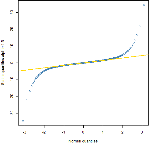
Figure 2: Quantile comparison of the normal and the stable distribution with alpha=1.8. 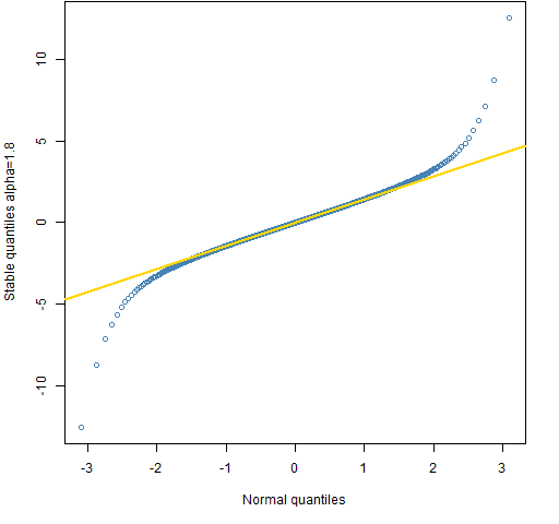
Figure 3: Quantile comparison of the normal and the stable distribution with alpha=1.9. 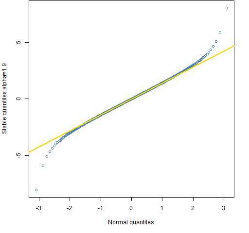
Figure 4: Quantile comparison of the normal and the stable distribution with alpha=1.95. 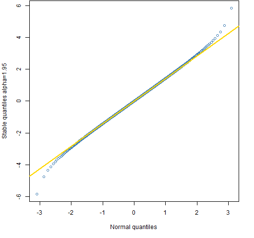
Questions
What benefits and demerits have I missed?
Summary
The stable distribution has a place in finance. That place should probably be smaller than the one envisioned by its keenest adherents.
Epilogue
were we the belly of the beast or the sword that fell…we’ll never tell.
from “The Stable Song” by Gregory Alan Isakov
Appendix R
The R language is one place you can find functionality for the stable distribution.
package
There are probably a few packages that include the stable distribution. A package that is dedicated to it is the stabledist package on CRAN. That is what is used for the plots.
plots
The function that created Figure 1 is:
P.stab15qqnorm <-
function (filename = "stab15qqnorm.png")
{
  if (length(filename)) {
    png(file = filename, width = 512)
    par(mar = c(5, 4, 0, 2) + 0.1)
  }
  s <- (1:999)/1000
  qs <- qstable(s, alpha=1.5, beta=0)
  plot(qnorm(s), qs, col="steelblue",
       xlab="Normal quantiles",
       ylab="Stable quantiles alpha=1.5")
  qqline(qs, datax=FALSE, lwd=2, col="gold")
  if (length(filename)) {
    dev.off()
  }
}
This function can be called with NULL as its argument to see the plot on the screen and correct what is wrong with it. Then calling it with no arguments creates the file that is actually used in the post.
The assumption of infinite variance is outright absurd from an empirical and economic point of view. The only amazing thing about stable distributions for me is that they still seem to be able to attract some followers and that their adherents (or maybe “disciples”?) are typically rather fierce believers.
Pingback: The scaling of Expected Shortfall | Portfolio Probe | Generate random portfolios. Fund management software by Burns Statistics
Pingback: Phân phối ổn định (Stable distribution) | MFEPE