More accurate than historical, simpler than garch.

Previously

We’ve discussed exponential smoothing in “Exponential decay models”.

The same portfolios were submitted to the same sort of analysis in “A look at historical Value at Risk”.

Issue

Markets experience volatility clustering.  As the previous post makes clear, historical VaR suffers dramatically from this.  An alternative is to use garch, the down-side of which is that it adds (some) complexity.  A middle ground is to use exponential smoothing: it captures quite a lot of the volatility clustering with a minimal increase in machinery.

Data

1000 long-only random portfolios were generated with exactly 60 stocks that had a maximum weight of 4% at the point when the portfolios were created (the end of 2006).  The universe was almost all of the constituents of the S&P 500 at a particular point in time.

Daily VaR using 500 days was estimated for each available time.  The time period over which we have VaR estimates is the start of 2008 to a few days into 2012.  The estimate uses a value of lambda in the exponential smooth of 0.97.  A t distribution is assumed with 7 degrees of freedom; the probability level is 5%.

Pictures

Figure 1 shows the fraction of times each of the 1000 portfolios experienced a hit.

Figure 1: Normal QQplot of the fraction of hits of the exponential smoothing VaR for 1000 random portfolios.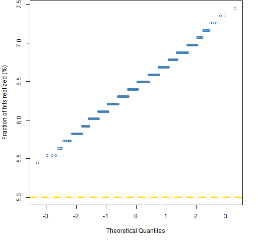

There are too many hits, but it is better than the comparable picture for historical VaR by about half a percent.  (See also “An infelicity with Value at Risk”.)

Figure 1 aggregates hits over time into one number for each portfolio.  Figure 2 aggregates hits over portfolios to get the fraction of portfolios hit on each day.  Some days are bad days and a lot of portfolios are hit, some days are good days and no portfolios are hit.

Figure 2: Fraction of portfolios that are hit with the exponential smoothing VaR on each day.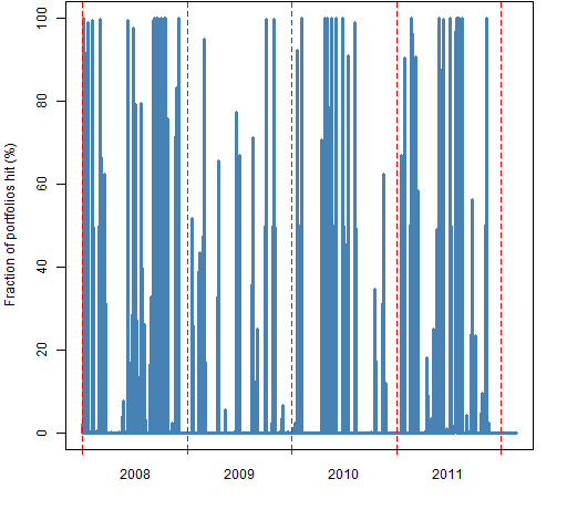

This looks much better than the corresponding picture for historical VaR.  Our eyes can detect clustering, but  we tend to interpret random data as clustered.  Figure 3 shows a random permutation of the data in Figure 2.

Figure 3: Randomly permuted fraction of portfolios that are hit on each day.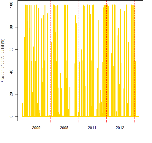

Testing autocorrelation of hits

We don’t have to depend on our eyes — we can do statistical tests to see if the hits are predictable or not.  One possibility is the Ljung-Box test.

Figure 4 shows the distribution across the portfolios of the p-value for a Ljung-Box test with 15 lags.

Figure 4: Distribution of the p-value of the Ljung-Box test with 15 lags for the hits of the exponential smooth VaR.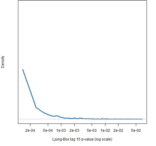

The p-values are all small, so we know there really is autocorrelation still left in the hits for the exponential smooth VaR.  However, these p-values are absolutely gigantic compared to the p-values for the historical VaR as shown in Figure 5.

Figure 5: Distribution of the base 10 logarithm of the p-value of the Ljung-Box test with 15 lags for the hits of the historical VaR.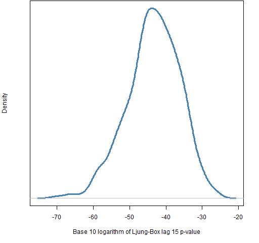

All the p-values here are zero for any practical purposes.

Summary

Exponential smoothing may be a good compromise between quality and complexity for Value at Risk.  As always, it depends on why you care.

Epilogue

Well I stumbled in the darkness
I’m lost and alone
Though I said I’d go before us
And show the way back home

from “Long Way Home” by Tom Waits and Kathleen Brennan

Appendix R

Computations were done in the R language.

Value at Risk computation

The function that does the actual VaR estimation was presented in “The estimation of Value at Risk and Expected Shortfall”.

The function is used multiple times to create a matrix of VaR estimates:

rp60texpsmo500VaR <- rp60ret
rp60texpsmo500VaR[] <- NA
vseq <- -500:-1
for(i in 501:1547) {
  tseq <- vseq + i
  for(j in 1:1000) {
    rp60texpsmo500VaR[i,j] <- VaRtExpsmo(rp60ret[tseq,j],
        digits=15)
  }
}

We start by creating a matrix the right size, filling it with missing values (mainly for safety but the first 500 rows remain missing), then filling in the values from the VaR estimation.

compute hits

Getting the hits is quite simple:

rp60texpsmo500hit <- rp60ret < -rp60texpsmo500VaR

Notice that this command highlights one of the few places in R where spaces make a difference.  (See Circle 8.1.30 of The R Inferno.)

aggregate hits

The hits are aggregated across time for each portfolio with:

rp60texpsmo500hitpmean <- apply(rp60texpsmo500hit, 
    2, mean, na.rm=TRUE)

qqnorm(rp60texpsmo500hitpmean)

The last command is a rough version of Figure 1.

Ljung-Box test

The p-values for the exponential smooth VaR are found with:

rp60texpsmo500lb15 <- apply(rp60texpsmo500hit, 2, 
   function(x) Box.test(as.numeric(x), type="Ljung", 
   lag=15)$p.value)

A function is created just for this occasion to coerce the data to numeric (from logical) and give back just the p-value from the test.  It is then used on each column (portfolio).

extracting tiny p-values

The result of the command above for the historical VaR can be more rapidly produced with:

rep(0, 1000)

The testing function rounds the p-values to zero.  We take the long way home:

rp60hist500lb15pvexp <- apply(rp60hist500hit, 2, 
   function(x) {
      st <- Box.test(as.numeric(x), type="Ljung", 
         lag=15)$statistic
      pchisq(st, df=15, lower=FALSE, log=TRUE) / 
         log(10)
   }
)

First we get the statistic for the test, which has a chi-squared distribution with degrees of freedom equal to the number of lags.  Then we get the (natural) logarithm of the upper tail for that statistic.  Finally we change the natural logarithm to base 10.