When investment skill is simulated, it is often presented as if it is obvious how to do it.  Maybe I’m wrong, but I don’t think it’s obvious.

Previously

In “Simple tests of predicted returns” we saw that prediction quality need not look like what you would find in a textbook.  For example, there was a case where there was no predictive power on the low values, but good prediction for high values.

Data

443 large cap US equities are used.  The variance matrix is estimated using the daily returns during 2011 (via a Ledoit-Wolf shrinkage model).

Both long-only and long-short portfolios are created.  The constraints for the long-only portfolios are:

• no more than 60 names in the portfolio
• predicted volatility is no more than 20%

The constraints for the long-short portfolios are:

• dollar neutral (net value of zero)
• no more than 60 names in the portfolio
• predicted volatility is no more than 10%

 

Simulating

There are unlimited ways of simulating skill.  Here we take a brief look at two.

Wilma

Wilma gets the correlation right (or wrong) separately for the halves of the data above and below the median of the realized values.  Three cases were created:

• the correlation is 10% for both halves (blue)
• the correlation is zero for the low half and 10% for the high half (gold)
• the correlation is -10% for the low half and 10% for the high half (black)

The colors indicate how the cases appear in the figures.  Figures 1 and 2 show the distributions of random portfolios generated using the three predictions plus a set that uses no predictions (colored green).

The sets of random portfolios use the predictions by having an extra constraint that the predicted return must be at least 90% of the way to the maximum predicted return.  In practice a fund manager is constrained by turnover considerations from moving to the best portfolio — the random portfolios are imitating this.

Figure 1: Distributions of 2012 Q1 returns for long-only portfolios: no prediction (green), Wilma 10,10 (blue), 0,10 (gold), -10,10 (black).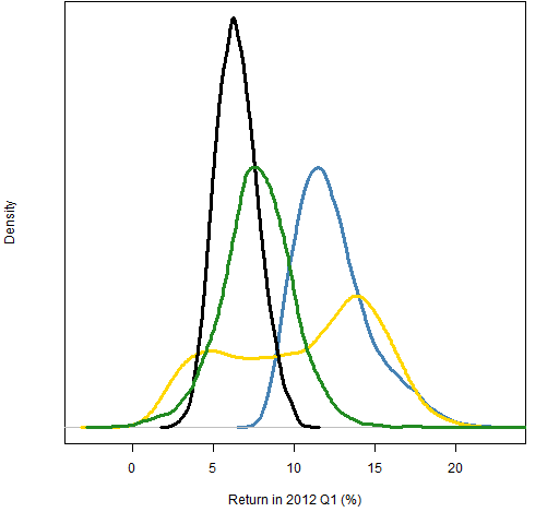

Figure 2: Distributions of 2012 Q1 returns for dollar-neutral portfolios: no prediction (green), Wilma 10,10 (blue), 0,10 (gold), -10,10 (black). 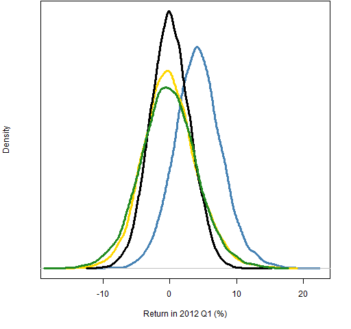Let’s focus on the blue distribution in Figures 1 and 2.  This is using one specific vector of predictions.  The variability is due to using that one prediction differently.  Think of it as Wilma having lots of different portfolios and using this one prediction vector to rebalance each of them.

But different prediction vectors with the same correlations may be more or less effective.  In fact, they can have significantly different correlations over the whole universe, as Figure 3 shows.

Figure 3: Correlation between realized and Wilma predictions where both halves have correlation 10%, with the correlation of the prediction used (blue). 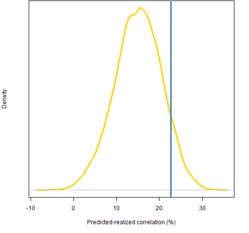The overall correlation is generally higher than 10% because the relationship is seen over a wider range.  But the overall correlation can be less than 10% as well by the lines having different slopes in the two halves.

Barney

Barney’s skill is different than Wilma’s.  Barney knows that a certain fraction of predictions and realized values match (or don’t match) in terms of being above or below their respective medians.  (This description is not quite accurate, and is probably hard to follow anyway — see the code in Appendix R  below for the real story.)

Again three predictions are used:

• 20% in each half are quaranteed to match (blue)
• 20% guaranteed to match in the high half (gold)
• 20% guaranteed not to match in the low half and 20% guaranteed to match in the high half (black)

Figures 4 and 5 show the returns of the random portfolios  using the same scheme of constraining the expected returns.

Figure 4: Distributions of 2012 Q1 returns for long-only portfolios: no prediction (green), Barney 20,20 (blue), 0,20 (gold), -20,20 (black).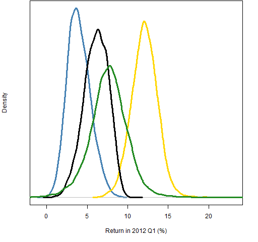

Figure 5: Distributions of 2012 Q1 returns for dollar neutral portfolios: no prediction (green), Barney 20,20 (blue), 0,20 (gold), -20,20 (black).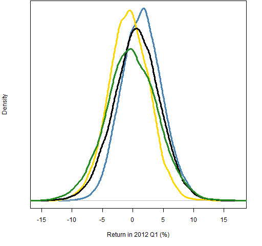 

Figure 5 is a mess in the sense that the differences between the distributions are subtle.  This is probably realistic.  The scheme from here would be to try to condition out more noise so that the effect of the prediction quality is more visible.

Figure 4 is a mess in the sense that it violates our expectations.  The supposedly best prediction does worst, and the supposedly mediocre prediction does very well.  One possibility is that there is a bug in the computations.  That shouldn’t be entirely ruled out, but there is a reasonable explanation for what we are seeing.

Figures 6 and 7 show the two predictions in question versus the realized returns.

Figure 6: Realized returns versus Barney predictions with 20% guarantee on the top half.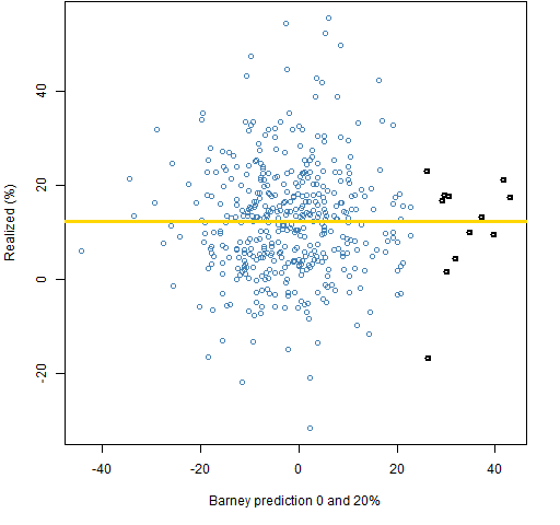

Figure 7: Realized returns versus Barney predictions with 20% guarantee on both halves. 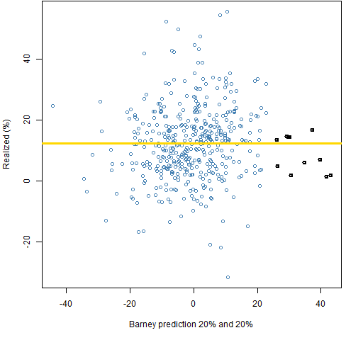Note in particular the highlighted points in Figures 6 and 7.  The most positive predictions are going to be the most important in long-only portfolios.  The center does not hold.  The 0-20 prediction has relatively good predictions in the tail, while the 20-20 has rather poor predictions in the tail.

Notice that a bound on position size is not one of the constraints.  The two most extreme points in Figures 6 and 7 are likely to be driving a lot of the returns.

Summary

Simulating investment skill is feasible and probably quite useful when done well.  Doing it well is unlikely to be done in an afternoon.

The textbook measures of the quality of prediction are going to be inadequate.

Be careful of the most extreme predictions.

Epilogue

Surely some revelation is at hand

from “The Second Coming” by W. B. Yeats

Joni Mitchell’s version.

Appendix R

The computations were done with R.

Wilma

The function to do the Wilma prediction:

pp.wilma <- function(realized, predicted=NULL, 
   cors=c(.1, .1), tol=.01)
{
  # simulate investment skill by adjusting correlation

  # Placed in the public domain 2013 by Burns Statistics

  # Testing status: untested

  if(length(predicted)) {
    if(length(predicted) != length(realized)) {
      stop("'realized' and 'predicted' need to be the same length")
    }
    if(length(intersect(names(realized), names(predicted)))) {
      stop("'realized' and 'predicted' need to for the same assets")
    }
    predicted <- predicted[names(realized)]
  } else {
    predicted <- realized
    predicted[] <- sample(predicted)
  }
  rmed <- median(realized)
  low <- realized <= rmed

  sfun.cor <- function(w, real, pred, targetCor) {
    cor(real, w * real + (1 - w) * pred) - targetCor
  }

  wlow <- uniroot(sfun.cor, c(-1,1), tol=tol, 
     real=realized[low], pred=predicted[low], 
     targetCor=cors[1])$root
  predicted[low] <- wlow * realized[low] + (1 - wlow) * 
     predicted[low]
  whi <- uniroot(sfun.cor, c(-1,1), tol=tol, 
     real=realized[!low], pred=predicted[!low], 
     targetCor=cors[2])$root
  predicted[!low] <- whi * realized[!low] + (1 - whi) * 
     predicted[!low]

  predicted
}

The three predictions were created (the rough beast is born) with:

pw12q1.1010 <- pp.wilma(real12q1, cors=c(.1, .1))
pw12q1.0010 <- pp.wilma(real12q1, cors=c(0, .1))
pw12q1.n1010 <- pp.wilma(real12q1, cors=c(-.1, .1))

Barney

The function to do the Barney prediction:

pp.barney <- function(realized, predicted=NULL, 
   fraction=c(.1, .1))
{
  # simulate investment skill by adjusting signs of predictions

  # Placed in the public domain 2013 by Burns Statistics

  # Testing status: untested

  if(length(predicted)) {
    if(length(predicted) != length(realized)) {
      stop("'realized' and 'predicted' need to be the same length")
    }
    if(length(intersect(names(realized), names(predicted)))) {
      stop("'realized' and 'predicted' need to for the same assets")
    }
    predicted <- predicted[names(realized)]
  } else {
    predicted <- realized
    predicted[] <- sample(predicted)
  }

  srmed <- sign(realized - median(realized))
  predicted <- predicted - median(predicted)
  lowi <- which(predicted < 0)
  hii <- which(predicted >= 0)
  changelow <- sample(lowi, round(abs(fraction[1]) * 
     length(lowi)),replace=FALSE)
  if(fraction[1] < 0) {
    predicted[changelow] <- -srmed[changelow] * 
      abs(predicted[changelow])
  } else if(fraction[1] > 0) {
    predicted[changelow] <- srmed[changelow] * 
      abs(predicted[changelow])
  }
  changehi <- sample(hii, round(abs(fraction[2]) * 
     length(hii)), replace=FALSE)
  if(fraction[2] < 0) {
    predicted[changehi] <- -srmed[changehi] * 
      abs(predicted[changehi])
  } else if(fraction[2] > 0) {
    predicted[changehi] <- srmed[changehi] * 
      abs(predicted[changehi])
  }

  predicted
}

The three predictions were created with:

pb12q1.2020 <- pp.barney(real12q1, fraction=c(.2, .2))
pb12q1.0020 <- pp.barney(real12q1, fraction=c(0, .2))
pb12q1.n2020 <- pp.barney(real12q1, fraction=c(-.2, .2))

estimate variance matrix

The variance estimate uses 250 daily returns in 2011:

require(BurStFin)
lwvar11 <- var.shrink.eqcor(initret[seq(to=2014,
   length=250), ])

allowable volatility

The rest of the computations depend on Portfolio Probe:

require(PortfolioProbe)

The first thing to do is to get the minimum variance portfolio with the constraints that we are using so that we will know how much volatility we need to allow for:

op.minvar.lo <- trade.optimizer(prices=initclose[2015,],
   variance=lwvar11, gross=1e7, long.only=TRUE, 
   port.size=60)

The predicted volatility of the minimum variance portfolio is:

> sqrt(252 * op.minvar.lo$var.value) 
[1] 0.133833

We can comfortably have 20% volatility in our portfolios.

allowable predicted return

The next step is to see what the best predicted expected return is given the constraints by doing another optimization:

op.pw1010.lo <- trade.optimizer(prices=initclose[2015,],
   variance=lwvar11, expected.return=pw12q1.1010, 
   gross=1e7, long.only=TRUE, port.size=60,
   var.constraint=.2^2/252)

The expected return of the optimal portfolio is in the alpha.value component of the resulting object, but we don’t really need to look at it in this case.  Optimizations were also done with the other prediction vectors.

We also do this for a dollar neutral portfolio where we limit volatility to 10%:

op.pw1010.ls <- trade.optimizer(prices=initclose[2015,], 
   variance=lwvar11, expected.return=pw12q1.1010, 
   gross=1e7, net=0, port.size=60,
   var.constraint=.1^2/252)

generate random portfolios

We start by generating random portfolios (10,000 in each go) with the same constraints as the optimizations:

rpvclo <- random.portfolio(number.rand=1e4, 
   prices=initclose[2015,], variance=lwvar11,
   gross=1e7, long.only=TRUE, port.size=60,
   var.constraint=.2^2/252)
rpvcls <- random.portfolio(number.rand=1e4, 
   prices=initclose[2015,], variance=lwvar11,
   gross=1e7, net=0, port.size=60,
   var.constraint=.1^2/252)

Now we generate random portfolios with these constraints plus a constraint on the expected return:

rp.pw1010.lo <- random.portfolio(number.rand=1e4, 
   prices=initclose[2015,], variance=lwvar11,
   expected.return=pw12q1.1010, 
   gross=1e7, long.only=TRUE, port.size=60,
   var.constraint=.2^2/252,
   alpha.constraint=unname(mean(pw12q1.1010) + .9 *
      (op.pw1010.lo$alpha.value - mean(pw12q1.1010))))

The alpha constraint is simpler in the dollar neutral case because we know that we expect zero when no prediction is used.

get returns

The only other operation of note is getting the returns of the random portfolios over the quarter of interest.  Really only the density of the returns is used:

density(100 * valuation(rp.pw1010.lo, 
   prices=initclose[c(2015, 2078),], returns='simple'))

This uses the valuation function from Portfolio Probe where the prices at the start and finish of the quarter are given and simple returns are asked for.