More efficiency and an additional function in the new version on CRAN.

Variance estimation

The major functionality in the package is variance estimation:

• Ledoit-Wolf shrinkage via var.shrink.eqcor
• statistical factor model (principal components) via factor.model.stat

There have been a number of previous blog posts on both factor models and Ledoit-Wolf shrinkage.

Positive-definiteness

The default value of the tol argument to var.shrink.eqcor is different in the new version.  The blog post “Correlations and positive-definiteness” suggested that the previous default was too extreme.

In finance we almost always want a variance matrix to definitely be positive-definite.  This is especially true when doing optimization.  Positive-definite means that all eigenvalues are greater than zero.  The tol argument in var.shrink.eqcor gives the minimum size of an eigenvalue in the result relative to the largest eigenvalue.

An eigenvalue of zero means that the variance matrix is saying that there is a portfolio (described by the corresponding eigenvector) that has zero variance.  An optimizer is going to really, really like such a portfolio — who wouldn’t?

The previous default for tol was 0.001.  The new default is 0.0001.  This is still a guess, but hopefully a more appropriate guess.

Efficiency

Both the input matrix and the resulting variance matrix can be large.  Financial applications often have a few thousand assets in a variance.  If there are multiple copies of these large objects within the function evaluation, that can be enough to push memory use over the limit in a computation.

Originally var.shrink.eqcor and factor.model.stat were written to get the computations right rather than worrying about memory or time efficiency.  (That’s the right order in which to worry.)  The new version uses fewer copies of the large objects.  That change accidentally sped up factor.model.stat a little.

If you run out of memory using one of these two functions, then:

First consider moving to 64-bit if you are still using 32-bit — R runs the same on either.  If you are on 64-bit already, consider getting more RAM (an application of Uwe’s maxim).

Next, you could try to make your code more efficient.  In particular, avoid Circle 2 of The R Inferno.

If none of that is applicable, then you may want to take evasive action.  var.shrink.eqcor uses more memory than factor.model.stat.  If you run out of memory with factor.model.stat, then you can set iter.max=0 to save some memory (and time) at the expense of a (probably) slightly worse estimate.

 Weird data

Real data (financial and other) tend not to be nice textbook examples.  Often there are missing values.  In finance we even want to have variables (assets) in a variance matrix that have no data at all.

One of many possible data glitches in finance is for a price to get stuck on one value.  This translates to returns that are all zero.  Zero is an underestimate of the variance of an asset, and most likely suggests there is a data problem.  But that isn’t true of all settings.  factor.model.stat has an argument called constant.returns.okay.  The new version produces a different — that is, not backward-compatible — result when this argument is TRUE (which is not the default).

It is reasonable to view the previous behavior regarding this argument to be a bug:  All correlations involving the variable are zero and the variance is a certain quantile of the variances of the other variables.  The new behavior is to set the variance to zero as well.

Probably the best thing to do when confronted with this is to set the constant returns to missing values.

A possible self-inflicted weirdness is to give the variance estimators prices rather than returns.  By default the functions produce a warning if the input data are all non-negative.

Time weights

Financial markets are dynamic.  That means that old data goes stale.  The most typical approach to this problem is to equally weight some number of the most recent observations.  The default weighting in var.shrink.eqcor and factor.model.stat is to linearly decrease weights in such a way that the oldest observation given has one-third the weight of the most recent.

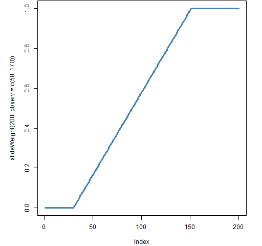
The new function in the package, called slideWeight, allows both of these, plus compromises between them.  The typical shape of weights from this function is shown in Figure 1.

Figure 1: Slide weights where 50 observations have full weight and 170 have some weight. 

The slideWeight function lets you specify a certain number of observations to have full weight, and a value beyond which all weights are zero.  The weights fall linearly between these two points.

See also

If you are new to R, learning R may be easier than you think.