What effect do predicted correlations have when optimizing trades?
Background
A concern about optimization that is not one of “The top 7 portfolio optimization problems” is that correlations spike during a crisis which is when you most want optimization to work.
This post looks at a small piece of that question. It wonders if increasing predicted correlations will improve the optimization experience during a crisis (when correlations do rise).
Data and portfolios
The universe is 443 large cap US stocks. We act as if we are optimizing as of 2008 August 29. 250 days of returns are used to estimate the variance matrix, and the next 60 days of prices are used to calculate the realized volatility.
The portfolios that were formed had constraints:
- long-only
- no more than 100 names
- no asset with more than 3% weight
Modifying correlations
You can get a sense of the average correlation during this time from Figures 1 and 2 of “S&P 500 correlations up to date”.
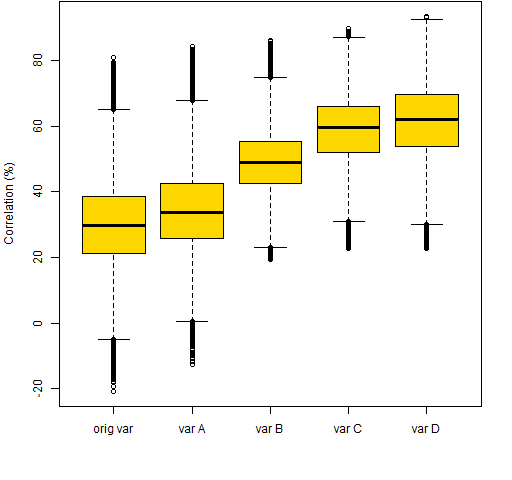
Ledoit-Wolf shrinkage goes towards the average estimated correlation. Here we have modified this so that there is shrinkage towards larger values of correlation. Figure 1 shows the distributions of correlations in the original Ledoit-Wolf estimate, and the four modified variances.
Figure 1: Predicted stock correlations within the five variance matrices.  It was harder than expected to force larger correlations in this way — see Appendix R for details.
Realized volatility
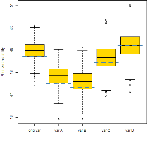
One reasonable test of the quality of a predicted variance matrix in this context is the realized volatility when the predicted portfolio variance is minimized. The results of the optimized portfolio can be noisy — hence not dependable — so for each variance estimate 1000 random portfolios were generated with predicted portfolio variance no more than 1.01 times that of the minimum variance portfolio.
Figure 2 shows the realized volatilities of the random portfolios.
Figure 2: Realized volatilities of the random portfolios (boxplots) and the minimum variance portfolio (blue).  There’s some improvement with modest adjustment, but nothing spectacular.
What’s missing?
In order to think that we know something, we’d want to have a better sense of the effect across different times and with different constraints.
In particular, we would want to see what happens when we bias correlations up, but they actually fall for the realized period.
Questions
Surely there are better ways to get bigger correlations. What are they?
Summary
This might be a path to pursue, but improvement is likely to be marginal. However, trying to understand the bigger picture definitely seems like a good thing to me.
Appendix R
Computations were done in R.
adjust Ledoit-Wolf: modify code
The var.shrink.eqcor function in the BurStFin package does Ledoit-Wolf shrinkage. One of the great things about R is that if a function does almost what you want, it is often easy to make a modified version that does exactly what you want.
A function (called var.shrink.eqcorMod) was created that has an extra argument called correlation that defaults to NULL. Then a section of code was added just before ans is created:
if(length(correlation)) {
  if(is.numeric(correlation) &&
      length(correlation) == 1) {
    if(verbose) {
       cat("original mean correlation is", meancor, "\n")
     }
   } else {
     cat("original mean correlation is", meancor, "\n",
         "Type in desired correlation:\n")
     correlation <- as.numeric(readline())
   }
   prior[] <- correlation
   diag(prior) <- 1
   prior <- sdiag * prior * rep(sdiag, each = nassets)
 }
So the user can either put in a correlation value from the start, or wait to see what would be shrunk towards without intervention.
adjust Ledoit-Wolf: doing it
The variance matrices were created by:
origvar <- var.shrink.eqcor(retmatPre08Aug)
modvarA <- var.shrink.eqcorMod(retmatPre08Aug,
   correlation=.9)
modvarB <- var.shrink.eqcorMod(retmatPre08Aug,
   correlation=.9, shrink=.5)
modvarC <- var.shrink.eqcorMod(retmatPre08Aug,
   correlation=.95, shrink=.8)
modvarD <- var.shrink.eqcorMod(retmatPre08Aug,
   correlation=.99, shrink=.99)
The shrinkage in the original variance is about 0.125.
correlation distribution
The code to produce Figure 1 was:
 mc <- function(x) 100 * cov2cor(x)[lower.tri(x)]
 boxplot(list("orig var"=mc(origvar), "var A"=mc(modvarA),
              "var B"=mc(modvarB), "var C"=mc(modvarC),
              "var D"=mc(modvarD)), col="gold",
              ylab="Correlation (%)")
optimize
The commands to do the optimization were like:
require(PortfolioProbe)
opA.lo.w03 <- trade.optimizer(price08Aug, modvarA,
   gross=1e6, long.only=TRUE, max.weight=.03,
   port.size=100, utility="minimum variance")
generate random portfolios
Generating the random portfolios is similar, except there is the additional constraint on the variance:
rpA.lo.w03 <- random.portfolio(1000, price08Aug, modvarA,
   gross=1e6, long.only=TRUE, max.weight=.03,
   port.size=100, utility="minimum variance",
   var.constraint=unname(opA.lo.w03$var.values * 1.01))
realized volatility
The realized volatility used in Figure 2 was computed like:
volA.lo.w03 <- apply(valuation(rpA.lo.w03,
   pricePost08Aug, returns="log"), 2, sd) * 100 *
   sqrt(252)
augment boxplot
The addition of information to boxplots as is done in Figure 2 is explained in “Variability of predicted portfolio volatility”.
