A prediction of a portfolio’s volatility is an estimate — how variable is that estimate?

Data

The universe is 453 large cap US stocks.

The variance matrices are estimated with the daily returns in 2012. Variance estimation was done with Ledoit-Wolf shrinkage (shrinking towards equal correlation).

Two sets of random portfolios were created.  In both cases the portfolios are long-only.  The first set has constraints:

• exactly 20 names in the portfolio and maximum weight of 8%

The second set has constraints:

• exactly 200 names and maximum weight of 2%

1000 portfolios were generated in each set.  Portfolios were formed as of the last trading day of 2012.

Figure 1 shows the distribution of predicted volatilities for the two sets of random portfolios.

Figure 1: Predicted volatility for two sets of 1000 random portfolios. 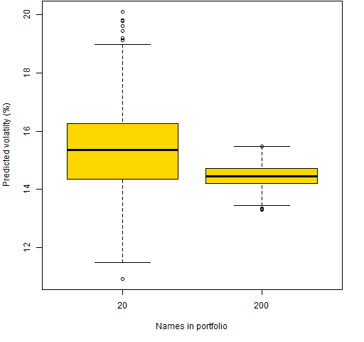The typical predicted volatility of the 200-name portfolios is slightly smaller than that for the 20-name portfolios.  The 20-name portfolios have a much wider range of predictions.

Prediction variability

The question we want to answer is: how variable is our estimate of the volatility for a specific portfolio.  Figure 1 shows variability across portfolios, we want instead to look at one particular portfolio at a time.

We create alternative estimates of the variance matrix using the statistical bootstrap.  The idea is to get estimates using data we might have seen rather than only looking at the estimate we get from the data we happened to have seen.

In what follows, we ignore almost all of the random portfolios and look at just the first 3 in each set.  Figure 2 shows the bootstrap distributions of the first three random portfolios with 20 names, and Figure 3 shows the same thing for the first 3 200-name portfolios.  100 bootstrap variance matrices were created.

Figure 2: Bootstrap distributions of three 20-name portfolios, actual estimate in blue.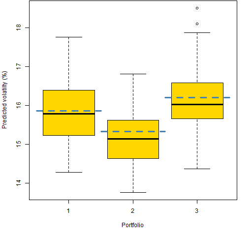

Figure 3: Bootstrap distributions of three 200-name portfolios, actual estimate in blue.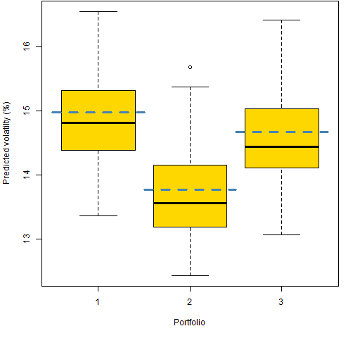

Figures 4 and 5 show the portfolio volatilities from each bootstrapped variance.

Figure 4: Predicted volatility of three 20-name portfolios from 100 bootstrapped variances.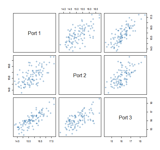

Figure 5: Predicted volatility of three 200-name portfolios from 100 bootstrapped variances. 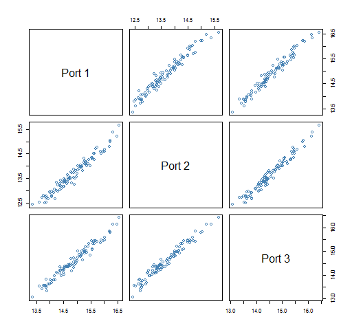In the 200-name portfolios each bootstrapped variance has about the same effect on each portfolio volatility estimate.  But in the 20-name portfolios a given bootstrapped variance matrix might produce a lower than average volatility estimate for one portfolio but a higher than average estimate for another portfolio.

What’s wrong?

The variability we are seeing is only from the noisiness of the data going into the variance estimate.  Implicitly it assumes that the process in the future will be the same as during the estimation period.  In finance that is a bad assumption.

The bootstrap distribution only provides a lower bound on the true variability.

Questions

Why are the original portfolio volatility estimates substantially bigger than the median of the bootstrapped values (Figures 2 and 3)?

Summary

Predictions have estimation error.  Danielsson and Macrae suggest that stating the variability of risk estimates should be standard.  I agree.

Epilogue

A temporary refuge where somebody else can stand

from “Night Train” by Bruce Cockburn

Appendix R

Here are R commands that were used.

estimate variance matrix

There is a function in the BurStFin package for Ledoit-Wolf estimation:

require(BurStFin)
lw12 <- var.shrink.eqcor(ret12)

Here ret12 is the matrix of returns of the 2012 daily returns (days in rows with most recent last, and stocks in columns).

generate random portfolios

The random portfolios are generated with the Portfolio Probe software:

require(PortfolioProbe)
rp20w08 <- random.portfolio(1000, 
   prices=tail(close12, 1), gross=1e6, long.only=TRUE,
   max.weight=.08, port.size=c(20,20))
rp200w02 <- random.portfolio(1000, 
   prices=tail(close12, 1), gross=1e6, long.only=TRUE,
   max.weight=.02, port.size=c(200,200))

Each random portfolio object is basically just a list of the contents of portfolios.

predicted volatility of random portfolios

A small function was written to make it easy to get portfolio volatilities of random portfolios:

pp.rpvol <- function(rp, varmat, annualize=252)
{
  # placed in public domain 2013 by Burns Statistics

  # testing status: untested

  rpvar <- unlist(randport.eval(rp, keep="var.values",
     additional.args=list(variance=varmat)), 
     use.names=FALSE)
  sqrt(annualize * rpvar) * 100
}

randport.eval is a Portfolio Probe function used here to get the predicted portfolio variance for each random portfolio.

This is used like:

vol20orig <- pp.rpvol(rp20w08, lw12)
vol200orig <- pp.rpvol(rp200w02, lw12)

one bootstrap variance matrix

Another little function was written to create a boostrapped variance matrix:

pp.bootvar <- function(RETMAT, FUN=var.shrink.eqcor, 
   ...)
{
  # placed in public domain 2013 by Burns Statistics

  # testing status: untested

  FUN <- match.fun(FUN)
  nobs <- nrow(RETMAT)
  bootobs <- sort(sample(1:nobs, nobs, replace=TRUE))
  FUN(RETMAT[bootobs,], ...)
}

This uses a few R tricks.

It might have struck you that the argument names are in all capitals — which goes against the grain.  This is to minimize the possibility of a collision between the arguments in this function and the arguments to the estimation function that are passed in via the three-dots argument.

Using match.fun is an easy way to get flexibility.  If FUN is a function, then it just returns that.  If FUN is a string, then it goes off and looks for a function by that name.

Usually the order of observations doesn’t matter.  However, the default for var.shrink.eqcor is to weight more recent observations more heavily.  Hence sorting the observations is a reasonable thing to do here.

bootstrapping portfolio volatilities

To see what is in Figures 4 and 5, we want to have results for a single bootstrapped variance matrix for each portfolio.  We also want to minimize the number of times we bootstrap a variance matrix because estimating the variance matrix is the most expensive part.

Hence we set up objects to hold the portfolio volatilities and then do the bootstrapping:

vol20boot <- vol200boot <- array(NA, c(100,3))
for(i in 1:100) {
  thislw <- pp.bootvar(ret12)
  vol20boot[i,] <- pp.rpvol(head(rp20w08, 3), thislw)
  vol200boot[i,] <- pp.rpvol(head(rp200w02, 3), thislw)
  cat("done with", i, date(), "\n")
}

You might think that a simplification would be to write:

rp20w08[1:3]

instead of:

head(rp20w08, 3)

You would be wrong.  The subscripting strips attributes.  But there is a head method for random portfolios that preserves the class attribute (and more).  The pp.rpvol function wouldn’t work if we just subscripted.

boxplots

Figure 2 was created with:

boxplot(vol20boot, col='gold', xlab="Portfolio", 
   ylab="Predicted volatilty (%)")
segments(x0=1:3 - .5, y0=vol20orig[1:3], x1=1:3 + .5,
   col="steelblue", lwd=3, lty=2)

The segments command uses the fact that the boxplots are centered at integers.

pairs plots

Figure 4 was made with:

pairs(vol20boot, col='steelblue', 
   label=paste("Port", 1:3))