How to capture return variability when testing strategies with long-short deciles.

Traditional practice

Question: Does variable X have predictive power for our universe of assets?

A common scheme of quants to answer the question is to form a series of portfolios over time.  The portfolio at each time point:

• is long the equal weighting of the assets in the top decile
• is short the equal weighting of the assets in the bottom decile

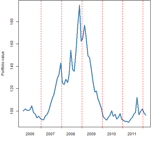
Figure 1 is an example.  It uses the default signal from the MACD function in the TTR R package.  The data are monthly for 474 large US equities.  So the deciles each have 47 stocks in them.

Figure 1: Efficacy of MACD via long-short deciles.

This test is acknowledged to be unrealistic in terms of turnover.  There seems to be no acknowledgement of the irony that quants — whose primary remit is understanding variability — are here sweeping all the variability under the carpet.

Adding variability

If instead of equal weighting, the assets in the deciles (or quintiles or whatever) are unequally weighted, then the answer will be different.

A way to get a different path through time is:

• create a set of weights in some range that sum to 1
• at each time point:
  • randomly assign weights for the long assets
  • randomly assign weights for the short assets

Then repeat that as many times as you like — 1000 times is done here.

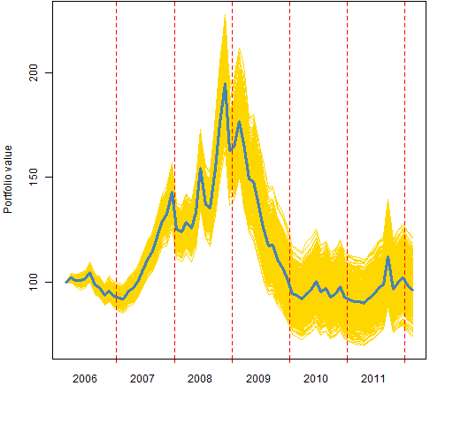
Figure 2 shows the variability of the MACD signal when the weights range  approximately from one-half to twice as big as the equal weight.

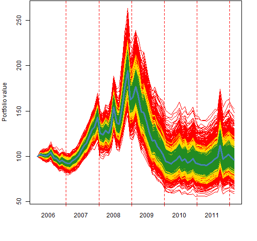
Figure 2: Efficacy of MACD via long-short deciles with weights that vary from about 0.5 to 2 times equal weighting. Figure 3 shows the variability when there are three different spreads for the weights.

Figure 3: Efficacy of MACD via long-short deciles with weights that vary from equal weighting by about: 0.66 to 1.5 times (green), 0.5 to 2 times (gold), 0.25 to 4 times (red).

Comment

This is a use of random portfolios.  However, the constraints are simple enough that there is no need for specialized software to generate the random portfolios.

Questions

What improvements can be made to this scheme?

Summary

It is easy to include variability in decile tests by using random weights.  Hence it probably should be.

Updates

2012 December 6: A simpler, and I think better, approach is given in “Again with long-short decile tests”.

Appendix R

The computations were done in R.

original computation

The command that gave the results shown in Figures 1 and 2 was:

macdDecitest2 <- pp.decileTest(sp5.macd[month.chuse,], 
    sp5.close[month.chuse,], wtspread=2)

additional computation

Because the result of pp.decileTest is a list with an appropriate call component, we can create variations of the object by using the update function and giving it the arguments that we want to change:

macdDecitest1.5 <- update(macdDecitest2, wtspread=1.5)
macdDecitest4 <- update(macdDecitest2, wtspread=4)

time plot

The plotting function depends on the pp.timeplot function.  This can be put into your R environment with:

source('https://www.portfolioprobe.com/R/blog/pp.timeplot.R')

plotting

Figure 1 is created by:

plot(macdDecitest2, random=FALSE)

Figure 2 is created by:

plot(macdDecitest2, random=TRUE)

Figure 3 is created by:

plot(macdDecitest4, random=TRUE, 
   col=c("steelblue", "red"))
plot(macdDecitest2, random=TRUE, 
   col=c("steelblue", "gold"), add=TRUE)
plot(macdDecitest1.5, random=TRUE, 
    col=c("steelblue", "forestgreen"), add=TRUE)
plot(macdDecitest4, random=FALSE, 
    col=c("steelblue", "red"), add=TRUE)

object-orientation

The result of pp.decileTest has a class attribute.  That means that it fits into the object orientation scheme of R.  In particular, it means that it is possible for plot to know what to do with these objects.

computation function

First, a low-level function to get the deciles:

pp.topBottom <- 
  function(x, n=round(length(x)/10))
  {
    # return the names of the smallest and 
    # largest elements
    # by default it returns deciles

    # put in the public domain 2012 by Burns Statistics

    # testing status:
    # seems to work

    nxs <- names(sort(x)) # inefficient but effective
    list(top=tail(nxs, n), bottom=head(nxs, n))
  }

Here is the function that does the computation:

pp.decileTest <-
  function(signal, prices, trials=1000, wtspread=2, 
     groups=10)
  {
    # R function to test a signal via long-short deciles
    # put in the public domain 2012 by Burns Statistics

    # testing status:
    # seems to work

    stopifnot(all(dim(signal) == dim(prices)), 
        length(groups) == 1, 
        identical(sort(colnames(signal)), 
        sort(colnames(prices))))

    ntimes <- nrow(prices)
    eqwtval <- rep(NA, ntimes)
    names(eqwtval) <- rownames(prices)
    randwtval <- array(NA, c(length(eqwtval), trials),
                       list(names(eqwtval), NULL))
    uret <- tail(prices, -1) / head(prices, -1) - 1
    randwtval[1,] <- eqwtval[1] <- 100

    nside <- round(ncol(prices) / groups)

    if(trials) {
      stopifnot(wtspread > 0)
      if(wtspread < 1) wtspread <- 1/wtspread
      portwts <- exp(seq(log(1/wtspread), 
         log(wtspread), length=nside))
      portwts <- portwts / sum(portwts)
      tseq <- 1:trials
      t.eret <- numeric(trials)
    }

    for(i in 1:(ntimes-1)) {
      tb <- pp.topBottom(signal[i, ], n=nside)
      botret <- uret[i, tb$bottom]
      topret <- uret[i, tb$top]
      this.eret <- mean(topret) - mean(botret)
      eqwtval[i+1] <- eqwtval[i] * (1 + this.eret)
      if(trials) {
        for(j in tseq) {
          t.eret[j] <- sum(sample(portwts) * topret) - 
            sum(sample(portwts) * botret)
        }
        randwtval[i+1, ] <- randwtval[i, ] * 
            (1 + t.eret)
      }
    }
    ans <- list(equal.weight=eqwtval, 
       random.weight=randwtval, nside=nside, 
       call=match.call())
    class(ans) <- "SignalTest"
    ans
  }

This function is written with the assumption that the universe is stable over time.  A more careful implementation would check for missing values at each time point.  That may cause the size of the deciles to change, and hence the weights would need to be revised.

plot function

Here is the plot method for objects created by the function above:

plot.SignalTest <-
  function(x, random=TRUE, add=FALSE, 
      col=c("steelblue", "gold"), lwd=c(3,1), 
      ylab="Portfolio value", lty=1, ...) 
  {
    # plot method for result of pp.decileTest
    # put in the public domain 2012 by Burns Statistics

    # testing status:
    # seems to work

    if(add) {
      if(random) {
        matlines(x$random.weight, col=col[2], 
           lwd=lwd[2], lty=lty, ...)
      } else {
        lines(x$equal.weight, col=col[1], lwd=lwd[1], 
           lty=lty, ...)
      }

    } else {
      # initial top-level plot
      if(random) {
        pp.timeplot(cbind(x$equal.weight, 
            x$random.weight), col=col[2], lwd=lwd[2], 
            lty=lty, ylab=ylab, ...)
        lines(x$equal.weight, col=col[1], lwd=lwd[1])

      } else {
        pp.timeplot(x$equal.weight, col=col[1], 
            lwd=lwd[1], lty=lty, ylab=ylab, ...)
      }
    }
  }