Not exactly pin-point accuracy.

Previously

Two related posts are:

• A practical introduction to garch modeling
• garch and long tails

Experiment

1000 simulated return series were generated.  The garch(1,1) parameters were alpha=.07, beta=.925, omega=.01.  The asymptotic variance for this model is 2.  The half-life is about 138 days.

The simulated series used a Student’s t distribution with 7 degrees of freedom and each series contained 2000 observations.

Estimation scatter

Figure 1 shows the distribution of the alpha and beta estimates.

Figure 1: Smoothed scatterplot of the alpha and beta estimates. 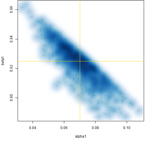Figure 1 makes more sense once we understand Figure 2, which shows the distribution of the estimated half-life.

Figure 2: Distribution of the estimated half-life. 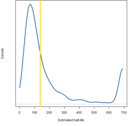The parameter constraints during the estimation means that the estimated half-life will be positive and will not exceed about 693 (the default constraint is alpha + beta < .999).  This explains why Figure 1 displays a sharpish top edge rather than the elliptical distribution we might expect.

Figure 3 shows how well the degrees of freedom are estimated, and Figure 4 shows the distribution of the estimated asymptotic variance.  The asymptotic variance (the predicted variance at an infinite horizon) for a garch(1,1) is omega / (1 – alpha – beta).

Figure 3: Distribution of estimated degrees of freedom.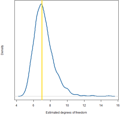

Figure 4: Distribution of estimated asymptotic variance.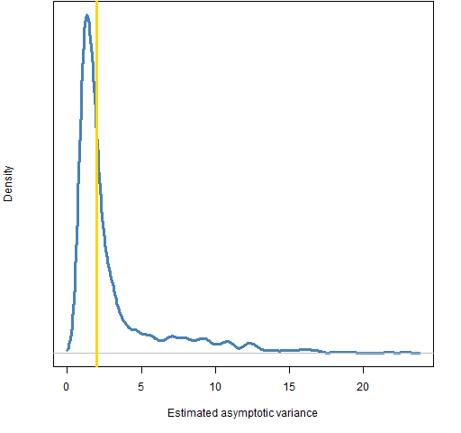

Summary

Even with 8 years of daily data, garch models are not precisely estimated.  Note that this is when we know the exact model.  Market data are not going to follow any model that we hypothesize.

This explains why there is not much value in garch predictions more than a few steps ahead.

Update: (2012 September 20) “garch estimates on impossibly long series” shows the results of the same experiment when the series each contain 100,000 observations.

Appendix R

The topics relating to R:

• the computations for this post
• simulating garch with the rugarch package
• simulating garch with the fGarch package

Post computations

simulate garch

Here is a function to simulate garch(1,1) series.  There are several ways to simulate garch already in R.  The advantage of this function is that it is easy to simulate with the parameters and distribution that you want.

pp.garchsim <- function(innov, 
    parameters=c(.01, .07, .925), varInit=NA, 
    tol=3/sqrt(n)) 
{
  # placed in the public domain 2012 by Burns Statistics
  # simulate a garch process
  #
  # test status: fit garch model to output and 
  # get similar parameters

  n <- length(innov)
  if(abs(var(innov) - 1) > tol) {
    warning("variance ",  var(innov), 
            " is farther from 1 than tolerance ", tol)
  }
  omega <- parameters[1]
  alpha <- parameters[2]
  beta <- parameters[3]
  if(is.na(varInit)) {
     varInit <- omega / (1 - alpha - beta)
  }
  varVec <- retVec <- numeric(n)
  varVec[1] <- varInit
  retVec[1] <- innov[1] * sqrt(varInit)
  # following loop assumes n > 1
  for(i in 2:n) {
    varVec[i] <- thisVar <- omega + alpha * 
      retVec[i-1]^2 + beta * varVec[i-1]
    retVec[i] <- innov[i] * sqrt(thisVar)
  }
  attr(retVec, "variance") <- varVec
  attr(retVec, "call") <- match.call()
  retVec
}

scale innovations

One of the assumptions with garch simulation is that the innovations have variance equal to 1.  So if you want to use t-distributed innovations, they need to be scaled.  The following function does that:

pp.rt <- function(n, df)
{
  # placed in the public domain 2012 by Burns Statistics
  # random Student's t generation scaled to variance 1
  #
  # testing status: seems to work
  sqrt((df - 2)/df) * rt(n, df)
}

If you fail to scale them, you can get explosive behavior as Figure 5 shows.  The call to create the data was:

gserExplode <- pp.garchsim(rt(2000, 5))

Figure 5: An explosive series.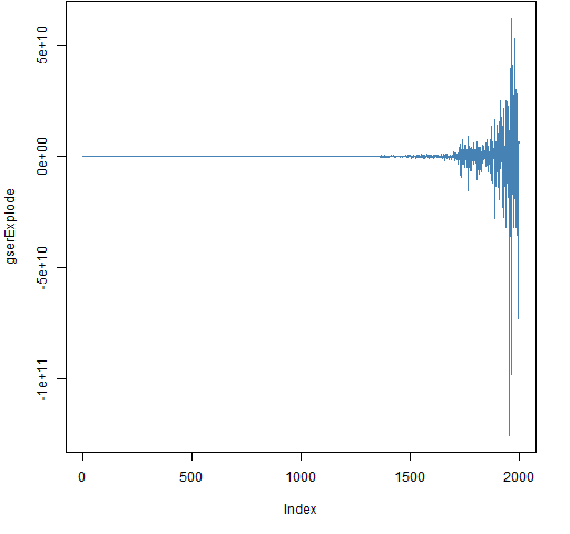

When the innovations have a non-unity variance then the true value of alpha is the given value times the innovation variance.  If that plus beta is greater than 1, then the series will be explosive.

estimate for the study

The function that did the set of estimations was:

pp.garchEstSim <- function(params, spec, 
   nobs=2000, df=7, trials=100)
{
  # placed in the public domain 2012 by Burns Statistics
  # estimates from simulated garch processes
  #
  # test status: not tested but seems to work

  require(rugarch)

  ret <- pp.garchsim(pp.rt(nobs, df))
  gco <- coef(ugarchfit(spec, ret))
  ans <- array(NA, c(trials, length(gco)), 
               list(NULL, names(gco)))
  ans[1,] <- gco

  # following loop assumes trials > 1
  for(i in 2:trials) {
    ret <- pp.garchsim(pp.rt(nobs, df))
    ans[i,] <- coef(ugarchfit(spec, ret))
  }
  attr(ans, "call") <- match.call()
  ans
}

The call to create the estimation data was:

tspec <- ugarchspec(mean.model=list(armaOrder=c(0,0)), 
   distribution="std")
system.time(ges.a.2000.07 <- pp.garchEstSim(
   c(.01, .07, .925), spec=tspec, nobs=2000, 
   df=7, trials=1000))

This started with trials=10 and then I decided how many series to generate given the approximate amount of time I was willing to wait.  The compute time for 1000 trials on my machine was about 700 seconds.

smooth scatterplot

Most of the plots in this blog are cleaned up versions of what I do for myself.  Figure 1 is an exception — it comes straight out of the box like that.  The two commands (using core functions) to create it are:

smoothScatter(ges.a.2000.07[,3:4])
abline(h=.925, v=.07, col="gold")

Simulate in rugarch

Simulation is easiest here on a fitted model.  So you might do something like:

tgarSeries20 <- pp.garchsim(pp.rt(2000, 20))
tgarFit20 <- ugarchfit(tspec, tgarSeries20)
tgarSim20 <- ugarchsim(tgarFit20, n.sim=4000)

There is a plot method for the simulation object:

> plot(tgarSim20)

Make a plot selection (or 0 to exit): 

1:   Conditional SD Simulation Path
2:   Return Series Simulation Path
3:   Conditional SD Simulation Density
4:   Return Series Simulation Path Density

Selection:

As you can see, it gives us a menu of choices.  So what if you just want  a specific plot?  The documentation for this is, let us say, sparse.  The answer (or at least an answer) is to give the number you want to the which argument:

plot(tgarSim20, which=1)

Simulate in fGarch

Simulation in this package is more conducive to specifying the parameters of the model that you want to simulate:

fgspec <- garchSpec(model=list(alpha=.07, 
   omega=.01, beta=.925))
fgsim <- garchSim(spec=fgspec, extended=TRUE, n=2000)

However, I wasn’t successful in seeing how to provide the simulation a specific set of innovations.