A look at return variability for portfolio changes.
The problem
Suppose we make some change to our portfolio. At a later date we can see if that change was good or bad for the portfolio return. Say, for instance, that it helped by 16 basis points. How do we properly account for variability in that 16 basis points?
Performance measurement
This is an exercise in performance measurement. We want to know: Was that a good decision?
One approach to performance measurement is to take the returns over the investigation period as fact and look at other possible decisions that could have been made.
Here we go the other way around. We take the decision as fact and think of the returns over the period as just one realization of a random process.
Supposings
Suppose we are holding a portfolio at the end of 2010, and it has the constraints:
- constituents from the S&P 500
- long-only
- at most 50 names
- no asset may account for more than 4% of the portfolio variance
Suppose further that the value of the portfolio is $10,000,000 and we are willing to trade $100,000 (buys plus sells).
The trade we did resulted in the return being larger by 16.28351 basis points during 2011 (not counting trading costs). But of course that is only how it happened to have turned out — history could have been different. A gain of 16.28351 basis points was not an inevitable result of that decision.
(It doesn’t really matter, but in the example presented here the initial portfolio is merely a random portfolio obeying the constraints, and the decision is to move towards smaller predicted variance.)
Bootstrapping
One way to assess variability is to use the statistical bootstrap. Figure 1 shows the bootstrap distribution of the return difference using daily data for the year.
Figure 1: Distribution of the return difference for the decision from bootstrapping daily returns in 2011. 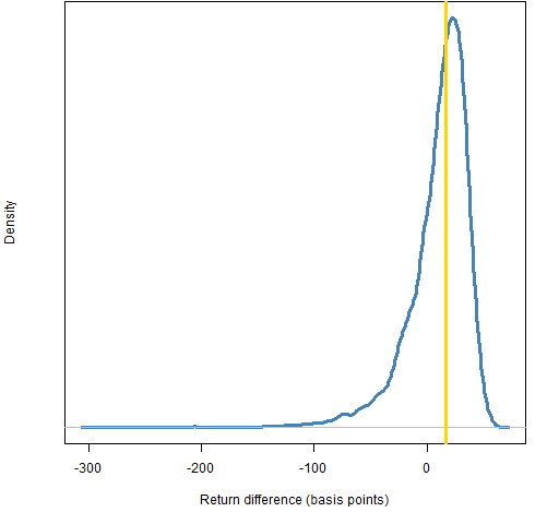 26% of the distribution in Figure 1 is below zero.
The bootstrap samples the days with replacement. It is (essentially) assuming that the returns are independent. That’s a quite strong assumption — it probably produces a distribution that is too variable.
We should be able to consider 26% as an upper limit on the p-value for the hypothesis that the difference is less than or equal to zero.
Figure 2 shows a typical case of the number of replicates for each value in a sample with 252 observations. Many observations (about a third) do not appear at all, and a few observations appear more than three times.
Figure 2: Number of replications for each observation in a bootstrap sample for 252 observations. 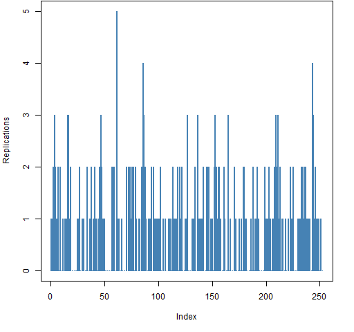
Jackknifing
The jackknife is generally considered to be a primitive version of the bootstrap. Another name for it is “leave-k-out”. The “k” is often 1. The equivalent of Figure 2 for the jackknife would be that all observations are at one replicate except for k at zero.
The jackknife disturbs the distribution much less — we’ll get less variability.
Figure 3 shows the return difference distribution from leaving out one daily return during the year.
Figure 3: Distribution of the return difference in 2011 for the decision from leaving out 1 daily return. 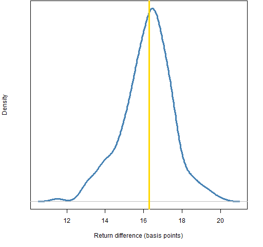
Figures 4 through 8 show the distributions from leaving out various fractions of the returns.
Figure 4: Distribution of the return difference in 2011 for the decision from leaving out 1% (that is, 3) of the daily returns. 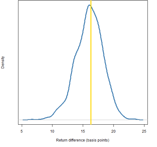
Figure 5: Distribution of the return difference in 2011 for the decision from leaving out 5% of the daily returns. 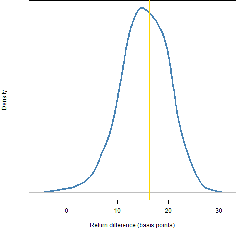
Figure 6: Distribution of the return difference in 2011 for the decision from leaving out 10% of the daily returns. 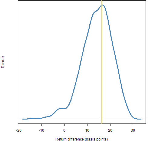
Figure 7: Distribution of the return difference in 2011 for the decision from leaving out 20% of the daily returns. 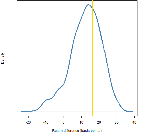
Figure 8: Distribution of the return difference in 2011 for the decision from leaving out 50% of the daily returns. 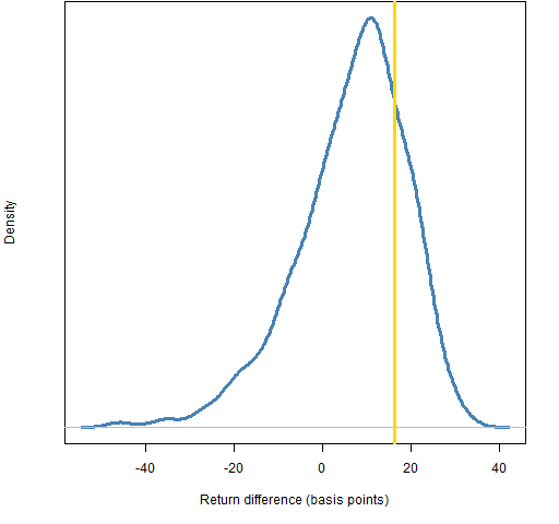 The fractions of the distributions below zero are: 0.5% for leave out 5%, 3% for leave out 10%, 9% for leave out 20%, and 26% for leave out 50%.
Questions
A quite interesting feature of Figure 1 is the long negative tail. Any ideas what is happening there? The trade closes MHS and opens WMT, but their return distributions for the year are both reasonably symmetric. The less symmetric MHS has a fairly trivial weight.
How can we decide what fraction of observations is best to leave out?
Have others done analyses similar to this?
Summary
If we could figure out how to determine the right amount of variability, this would be an interesting approach.
Epilogue
You’re old enough to make a choice
It’s just that in between all the words on the screen
I doubt you’ll ever hear a human voice
from “Walk Between the Raindrops” by James McMurtry
Appendix R
The computations were done with R.
replication plot
Figure 2 was produced like:
jjt <- table(sample(252, 252, replace=TRUE))
bootcount <- rep(0, 252)
names(bootcount) <- 1:252
bootcount[names(jjt)] <- jjt
plot(bootcount, type='h')
The type of the plot is ‘h’ for “high-density”. I’m not convinced I know why it is called that.
return difference
The function to compute the difference in returns between two portfolios is:
> pp.retdiff
function (wt1, wt2, logreturns)
{
        ret1 <- sum(wt1 * (exp(colSums(logreturns[,
                 names(wt1)])) - 1))
        ret2 <- sum(wt2 * (exp(colSums(logreturns[,
                 names(wt2)])) - 1))
        ret2 - ret1
}
This takes a matrix of log returns, sums them over times, then coverts to simple returns in order to multiply by the weights — see “A tale of two returns”.
jackknife
The function that was used to do the jackknifing was:
> pp.jackknife.rows
function (X, FUN, NOUT=1, FRACTION=NULL, TRIALS=1000, ...)
{
        nobs <- nrow(X)
        if(length(FRACTION) == 1) {
                NOUT <- max(1, round(nobs * FRACTION))
        } else if(length(FRACTION) > 1) {
                stop("'FRACTION' must have length 1 or 0")
        }
        if(is.character(FUN)) FUN <- get(FUN)
        if(!is.function(FUN)) {
                stop("'FUN' is not a function")
        }
        if(NOUT == 1) {
                ans <- numeric(nobs)
                for(i in 1:nobs) {
                        ans[i] <- FUN(X[-i,,
                             drop=FALSE], ...)
                }
        } else {
                ans <- numeric(TRIALS)
                for(i in 1:TRIALS) {
                        out <- sample(nobs, NOUT)
                        ans[i] <- FUN(X[-out,,
                             drop=FALSE], ...)
                }
        }
        ans
}
The arguments to this function will look really ugly to a lot of people. That’s sort of the point. It accepts a function as an argument and accepts additional arguments to that function via the three-dots construct. There is the possibility of a conflict of argument names. One convention for limiting that possibility is to use argument names in all capitals in functions with a function as an argument.
There are various ways of using these functions to do our jackknifing. Here is one way:
pp.jackknife.rows(sp5.logret11, pp.retdiff,
       wt1=jack.initwt, wt2=jack.optwt)
Here is another:
pp.jackknife.rows(sp5.logret11, function(x)
       pp.retdiff(jack.initwt, jack.optwt, x))
These do the same thing in different ways. The first gives the first two arguments of pp.retdiff by name. These are then the inhabitants of the three-dots inside pp.jackknife.rows. When pp.retdiff is called, the only unmatched argument is the third one, which is what we want.
The second method creates an anonymous function and passes it in as the FUN argument.
