All models are wrong, some models are more wrong than others.

The streetlight model

Exponential decay models are quite common.  But why?

One reason a model might be popular is that it contains a reasonable approximation to the mechanism that generates the data.  That is seriously unlikely in this case.

When it is dark and you’ve lost your keys, where do you look?  Under the streetlight.  You look there not because you think that’s the most likely spot for the keys to be; you look there because that is the only place you’ll find them if they are there.

Photo by takomabibelot via everystockphoto.com

Long ago and not so far away, I needed to compute the variance matrix of the returns of a few thousand stocks.  The machine that I had could hold three copies of the matrix but not much more.

An exponential decay model worked wonderfully in this situation.  The data I needed were:

• the previous day’s variance matrix
• the vector of yesterday’s returns

The operations were:

• do an outer product with the vector of returns
• do a weighted average of that outer product and the previous variance matrix

Compact and simple.

There are better ways, it’s just that the time was wrong.

The “right” way would be to use a long history of the returns of the stocks and fit a realistic model.  Even if that computer could have held the history of returns (probably not), it is unlikely it would have had room to work with it in order to come up with the answer.  Plus there would have been lots of data complications to work through with a more complex model.

“The shadows and light of models” used a different metaphor of light in relation to models.  If we can only use an exponential decay model, measuring ignorance is going to be a bit dodgy.  We won’t know how much of the ignorance is due to the model and how much is inherent.

Exponential smoothing

We can do exponential smoothing of the daily returns of the S&P 500 as an example.  Figure 1 shows the unsmoothed returns.  Figure 2 shows the exponential smooth with lambda equal to 0.97 — that is 97% weight on the previous smooth and 3% weight on the current point.  Figure 3 shows the exponential smooth with lambda equal to 1%.

Note: Often what is called lambda here is one minus lambda elsewhere.

Figure 1: Log returns of the S&P 500.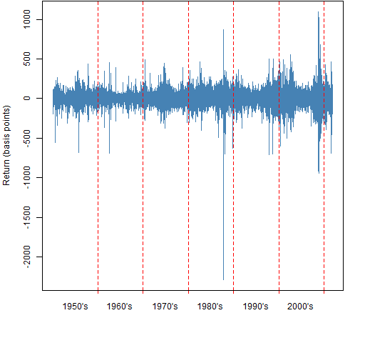

Figure 2: Exponential smooth of the log returns of the S&P 500 with lambda equal to 0.97.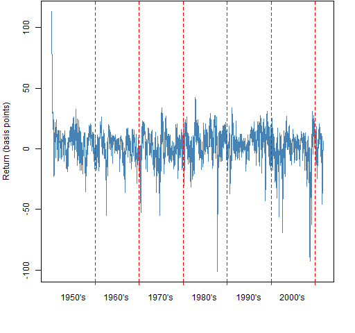

Figure 3: Exponential smooth of the log returns of the S&P 500 with lambda equal to 0.99.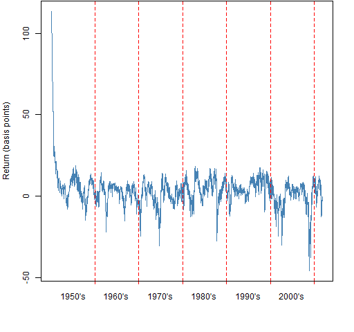

Notice that the start of the smooth in Figures 2 and 3 is a little strange.  The first point of the smooth is the actual first datapoint, which happened to be a little over 1%.  That problem can be solved by allowing a burn-in period — dropping the first 20, 50, 100 points in the smooth.

Chains of weights

The simple process of always doing a weighted sum of the previous smooth and the new data means that the smooth is actually a weighted sum of all the previous data with weights that decrease exponentially.  Figure 4 shows the weights that result from two choices of lambda.

Figure 4: Weights of lagged observations for lambda equal to 0.97 (blue) and 0.99 (gold). 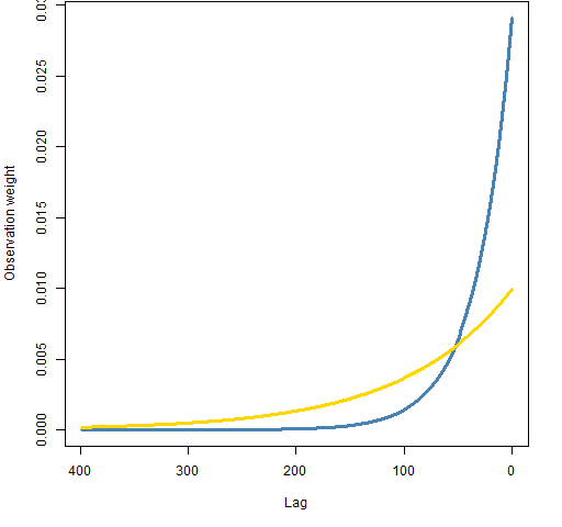The weights drop off quite fast.  If the process were stable, we would want the observations to be equally weighted.  It is easy to do that compactly as well:

• keep the sum of the statistic you want
• note the number of observations
• add the new statistic to the sum and divide by the number of observations

What we are likely to really want is some compromise between these extremes.

Half-life

The half-life of an exponential decay is often given.  This is the number of lags at which the weight falls to half of the weight for the current observation.  Figure 5 shows the half-lives for our two example lambdas.

Figure 5: Half-lives and weights of lagged observations for lambda equal to 0.97 (blue) and 0.99 (gold).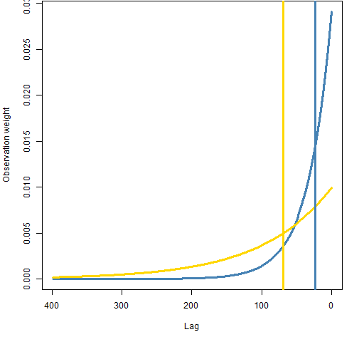

Generally the half-life is presented as if it is an intuitive value.  Well, sounds cool — I’m not sure it tells me much of anything.

Summary

When an exponential decay model is being used, you should ask:

Is there a good reason to use exponential decay, or is it only used because it has always been done like that?

Advances in hardware means that some of what could only be modeled with exponential decay in the past can now be modeled better.  It also means that what could not be done at all before can now be done with exponential decay.

Epilogue

He finds a convenient street light, steps out of the shade
Says something like, “You and me babe, how about it?”

from “Romeo and Juliet” by Mark Knopfler

Appendix R

R is, of course, a wonderful place to do modeling — exponential and other.

naive exponential smoothing

A naive implementation of exponential smoothing is:

> pp.naive.exponential.smooth
function (x, lambda=.97)
{
        ans <- x
        oneml <- 1 - lambda
        for(i in 2:length(x)) {
                ans[i] <- lambda * ans[i-1] + oneml * x[i]
        }
        ans
}

This is naive in at least two senses.

It does the looping explicitly.  For this simple case, there is an alternative.  However, in more complex situations it may be necessary to use a loop.

The function is also naive in assuming that the vector to be smoothed has at least two elements.

> pp.naive.exponential.smooth(100)
Error in ans[i] <- lambda * ans[i - 1] + oneml * x[i] :
  replacement has length zero

This sort of problem is a relative of Circle 8.1.60 in The R Inferno.

better exponential smoothing

Exponential smoothing can be done more efficiently by pushing the iteration down into a compiled language:

> pp.exponential.smooth
function (x, lambda=.97)
{
        xmod <- (1 - lambda) * x
        xmod[1] <- x[1]
        ans <- filter(xmod, lambda, method="recursive",
               sides=1)
        attributes(ans) <- attributes(x)
        ans
}

This still retains some naivety in that it doesn’t check that lambda is of length one.

See also the HoltWinters function in the stats package, and ets in the forecast package.

weight plots

A simplified version of part of Figure 5 is:

> plot(.03 * .97^(400:1), type="l", xaxt="n")
> axis(1, at=c(0, 100, 200, 300, 400),
+    labels=c(400, 300, 200, 100, 0))
> abline(v=400 - log(2) / .03)

time plot

The plots over time were produced with pp.timeplot.

Subscribe to the Portfolio Probe blog by Email