How many baskets are your eggs in?
Meucci diversity
Attilio Meucci directly addresses the adage:
Don’t put all your eggs in one basket.
His idea is to think of your portfolio as a set of subportfolios that are each uncorrelated with the rest. If your portfolio can be configured to have a lot of roughly equally weighted subportfolios, then your portfolio is well diversified.
Harald Lohre and Carsten Zimmer just put out a paper “Diversified Risk Parity Strategies for Equity Portfolio Selection” that discusses this topic. They show some results of applying the idea to the S&P 500.
Asset correlation to the portfolio
Another approach is to look at the eggs rather than the baskets.
We don’t want any asset to be overly correlated with our portfolio. If even one asset is highly correlated to the portfolio, then the portfolio can not be very diversified.
We can have a look at the asset-portfolio correlations by generating some random portfolios. We’ll use (almost all of) the S&P 500 constituents as of the start of 2011. We need a variance matrix of the assets as the basis of the correlation estimates. We use a Ledoit-Wolf shrinkage estimate based on daily data during 2010.
Our first set of portfolios obey the constraints:
- long-only
- exactly 20 names
- maximum weight is 10%
- minimum weight is 1%
Figure 1 shows the sorted asset-portfolio correlations for the portfolio that happened to be the first one computed.
Figure 1: Asset-portfolio correlations in a 20-name portfolio with weight constraints — blue are in the portfolio, gold are outside the portfolio. 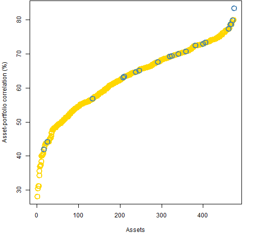 Figure 1 is quite typical. Figure 2 shows a case where several of the largest correlations are for stocks outside the portfolio.
Figure 2: Asset-portfolio correlations in a 20-name portfolio with weight constraints — blue are in the portfolio, gold are outside the portfolio. 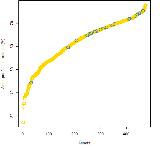
A second set of random portfolios was generated that obey the constraints:
- long-only
- exactly 200 names
- maximum weight is 1%
- minimum weight is 0.1%
Figure 3 shows correlations from the first of these portfolios.
Figure 3: Asset-portfolio correlations in a 200-name portfolio with weight constraints — blue are in the portfolio, gold are outside the portfolio. 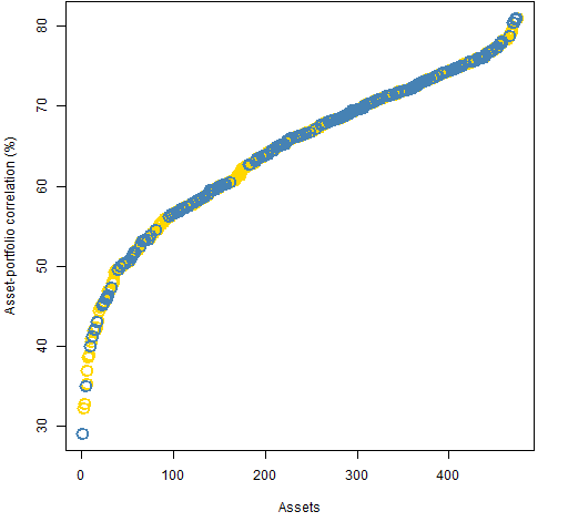 There are at least two things of note in Figure 3:
- The distribution of correlations is remarkably similar to that in the 20-name portfolios — we don’t seem to be gaining diversification with the extra names.
- The minimum correlation is for an asset that is in the portfolio.
Figure 4 shows the maximum correlation for each of the 1000 portfolios in each set.
Figure 4: QQ-plot of maximum correlation in each portfolio in two sets of random portfolios. 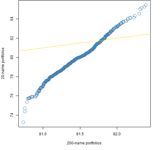 So, ironically, the 20-name portfolios tend to be more diversified — by this criterion — than the 200-name portfolios.
Constraining maximum correlation
Two additional sets of random portfolios were generated. The constraints are:
- long only
- exactly 20 names — or — exactly 200 names
- no asset may have a correlation with the portfolio greater than 60%
Weight constraints are redundant in this case, and perhaps counter-productive. Putting the maximum correlation at 50% seems to be too strong.
Figure 5 shows the asset-portfolio correlations for the first of the 20-name portfolios with the correlation constraint, and Figure 6 is for the first of the 200-name portfolios.
Figure 5: Asset-portfolio correlations in a 20-name portfolio with correlation constraint — blue are in the portfolio, gold are outside the portfolio. 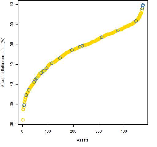
Figure 6: Asset-portfolio correlations in a 200-name portfolio with correlation constraint — blue are in the portfolio, gold are outside the portfolio. 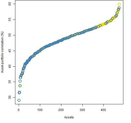 It seems to be a general feature for the 200-name correlation-constrained portfolios that the assets in the portfolio overwhelmingly have small correlations.
Questions
How are these two ideas of diversity — principal portfolios and asset-portfolio correlations — connected?
Summary
I hadn’t thought about asset-portfolio correlations very much before, but now I think they may have some serious promise.
That going from 20 to 200 names does not diversify in terms of correlations is quite interesting.
Epilogue
The most tender place in my heart is for strangers
I know it’s unkind but my own blood is much too dangerous
from “Hold On, Hold On” by Neko Case
Appendix R
R provided the computing and graphing environment.
generating random portfolios
The 20-name portfolios were generated by:
> require(PortfolioProbe)
> divrp.20w <- random.portfolio(1000, sp5.price10,
+    sp5.var10, gross=1e7, long.only=TRUE, max.weight=.1,
+    threshold=1e7 * .01/sp5.price10, port.size=c(20,20))
> divrp.20c60 <- random.portfolio(1000, sp5.price10,
+    sp5.var10, gross=1e7, long.only=TRUE,
+    rf.style="corport", risk.fraction=.6,
+    port.size=c(20,20))
collecting correlations
The randport.eval function in Portfolio Probe allows you to get pieces of the output for each random portfolio as if it had been optimized. In this case we want to get the risk.fraction component that holds the asset-portfolio correlations.
For the weight-constrained portfolios we need to add some arguments to the implicit optimization call in order for the correlations to be computed.
> divrp.20w.apcor <- randport.eval(divrp.20w,
+    keep="risk.fraction", additional.args=list(
+    rf.style="corport", risk.fraction=1))
> divrp.20c60.apcor <- randport.eval(divrp.20c60,
+    keep="risk.fraction")
collecting maximum correlations
In the previous step we created lists that are as long as the number of random portfolios (1000) containing the asset-portfolio correlations. Now instead of a vector of correlations for each portfolio, we want a single number for the portfolio — its maximum correlation.
> divrp.200w.apcormax <- sapply(divrp.200w.apcor,
+    function(x) max(x[[1]]))
> divrp.20w.apcormax <- sapply(divrp.20w.apcor,
+    function(x) max(x[[1]]))
The tricky part here is that each component of the lists is not a vector of correlations. Each component is a list whose first (and only) component is the correlations. Hence we need to select the first component before taking the maximum.
QQ-plot
The qqnorm function is familiar to a lot of R users. It compares some numeric data to the normal distribution.
Less familiar is the qqplot function. This compares the distributions of two datasets.
Figure 4 is essentially:
> qqplot(divrp.200w.apcormax, divrp.20w.apcormax)
> abline(0,1)
Pingback: Wednesday links: locked markets | Abnormal Returns
Pingback: Asset correlations with minimum variance portfolios | Portfolio Probe | Generate random portfolios. Fund management software by Burns Statistics
Pingback: Popular posts 2012 May | Portfolio Probe | Generate random portfolios. Fund management software by Burns Statistics
Pingback: 2 dimensions of portfolio diversity | Portfolio Probe | Generate random portfolios. Fund management software by Burns Statistics