A bit of testing of the estimation of the variance matrix for S&P 500 stocks in 2011.

Previously

There was a plot in “Realized efficient frontiers” showing the realized volatility in 2011 versus a prediction of volatility at the beginning of the year for a set of random portfolios.  A reader commented to me privately that they expected the plot not to be so elliptical — that they expected there to be higher dispersion for high volatility portfolios.

My initial hypothesis was that maybe the Ledoit-Wolf estimate is better than the factor models that the reader is used to.  We’ll test that and a few other hypotheses.

The realized period in this post is all of 2011.

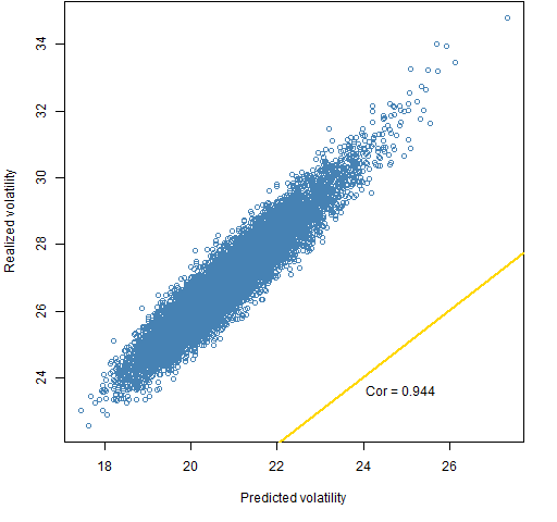
Figure 1 shows the realized and predicted volatility of 10,000 random portfolios.

Figure 1: Ledoit-Wolf estimate with linearly decreasing weights on a 1 year lookback for portfolios with risk fraction constraints. This shows the correlation among the random portfolios and the line where predicted and realized are equal.  Many tests of variance matrices use one portfolio and look at the vertical distance between that portfolio and the equality line.  That’s not really much of a test.

The future is very likely to be either more volatile or less volatile than the sample period.  The plots here suggest that getting the level right is just a matter of a single scaling parameter.

What is more important — certainly in the context of optimization — is knowing which of two portfolios will have the larger volatility.  That is, the correlation between realized and predicted is really of interest.

Estimators

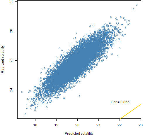
My hypothesis was that perhaps factor models wouldn’t be as good as Ledoit-Wolf shrinkage.  Figure 2 is the same as Figure 1 except that a statistical factor model is used instead of Ledoit-Wolf to predict volatility.

Figure 2: Statistical factor estimate with linearly decreasing weights on a 1 year lookback for portfolios with risk fraction constraints.

Figures 1 and 2 are close to identical with Ledoit-Wolf nosing out the statistical factor model.  It would be interesting to see results for other factor models.

Constraints

The random portfolios in Figures 1 and 2 were generated with the constraints:

• long-only
• 90 to 100 names
• no asset can contribute more than 3% to the portfolio variance

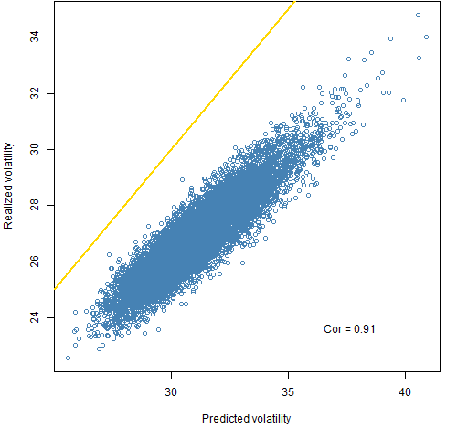
Figure 3 shows what happens when we replace the last constraint with:

• no asset can contribute more than 3% weight

Figure 3: Ledoit-Wolf estimate with linearly decreasing weights on a 1 year lookback for portfolios with weight constraints. Figure 3 has a much lower correlation than Figure 1.  However, that is not a general result.  The presentation “Portfolio optimisation inside out” shows a case where the weight constraints have a higher correlation than the corresponding risk fraction constraints.

An important difference in the present case is that the range of predicted volatilities is much narrower for the weight constraints, so it is natural for the correlation to be lower.

Time weights

It is possible to give more weight to some observations than others.  The default weighting in the variance estimators (Ledoit-Wolf and statistical factor) in the BurStFin package is linearly decreasing.  The most recent observation has 3 times the weight of the first observation in the sample period.  That is the weighting used in Figures 1 through 3.

Figure 4 uses equal weights for all the sample period, which is 2010.

Figure 4: Ledoit-Wolf estimate with equal weights on a 1 year lookback for portfolios with risk fraction constraints.

This is barely worse than using the linearly decreasing weights.

Lookback

The size of the sample period is an extreme form of controlling time weights.  The time weights of observations too far back in time are set to zero.

Figure 5: Ledoit-Wolf estimate with linearly decreasing weights on a 5 year lookback for portfolios with risk fraction constraints.

The five-year sample period is worse than the one-year period.

Caveat

You shouldn’t think that we’ve really learned anything here.  In order to get a firm sense of what works best we need to do this sort of thing over multiple times.  The market changes.  Different periods are different.  What we’ve seen here is just for one period.

However, for this one period the observations are:

• risk fraction constraints give higher correlation than weight constraints (this is known to be time-dependent, and in this case not a valid comparison of accuracy)
• 1-year lookback is better than 5-year lookback
• linearly decreasing weights are slightly better than equal weights
• Ledoit-Wolf shrinkage is slightly better than the statistical factor model

Summary

Using random portfolios to test variance matrix estimators provides vastly more useful information than the alternative.

The details of variance estimation seem to be fairly unimportant.  I of course mean within reasonable limits — the sample variance isn’t going to do when there are more assets than observations.

Questions

If we wanted to get a subset of the risk fraction random portfolios that had approximately the same distribution of predicted volatility as the weight constraint random portfolios, what would be a good way of selecting the subset?

Epilogue

It turned out to be the howling of a dog
Or a wolf, to be exact.
The sound sent shivers down my back

from “Furr” by Eric Earley

Appendix R

An explanation of the R computations is given in “Realized efficient frontiers” but a few extra things were done here.

The statistical factor model as well as the Ledoit-Wolf estimator is from the BurStFin package.

require(BurStFin)
var.sf.10.lw <- factor.model.stat(sp5.ret[1007:1258, ])

The command to get equal weights is:

var.lw.10.qw <- var.shrink.eqcor(sp5.ret[1007:1258, ], weight=rep(1,252))

safety tip

This analysis involved two sets of random portfolios.  It would be easy to mix objects concerning the two sets.  But there is a trick to reduce that possibility.

The first set of random portfolios contained 10,000 portfolios.  The second was created to have 10,001 portfolios.  Mixing up objects in this case is very likely to produce either an error or a warning.

Subscribe to the Portfolio Probe blog by Email