A look at the distortion from predicted to realized.

The idea

The efficient frontier is a mainstay of academic quant.  I’ve made fun of it before.  This post explores the efficient frontier in a slightly less snarky fashion.

Data

The universe is 474 stocks in the S&P 500.  The predictions are made using data from 2010.  The realized period is 2011.

The return predictor is MACD — essentially a momentum estimate.  As before this is used neither to praise nor to denigrate it, but rather because it is a publicly available method that is sometimes effective.

The variance matrix is estimated via Ledoit-Wolf shrinkage towards equal correlation.

Constraints

The efficient frontier is a function of the constraints.  We’ll use one set of constraints here:

• long-only
• 90 to 100 names in the portfolio
• no more than 3% of the portfolio variance attributed to any asset

Prediction

Figure 1 shows the predictions for 10,000 random portfolios that obey the constraints — the plot uses efficient frontier style axes.  (In this case the return predictor isn’t literally predicting returns, but something thought to be correlated with returns.)

Figure 1: Return prediction versus predicted volatility of 10,000 random portfolios.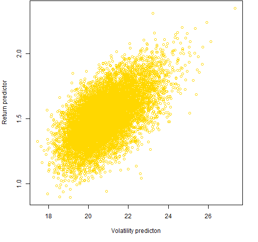

I was surprised at the shape of Figure 1.  I expected a fan shape — a wider range of return predictions for higher volatility portfolios.  My expectation is reinforced by looking at this relationship for the assets (Figure 2).

Figure 2: Return prediction versus predicted volatility for the individual stocks.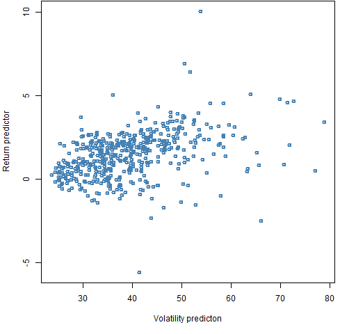

Figure 3 adds a few points on the efficient frontier to what is plotted in Figure 1.

Figure 3: Return prediction versus predicted volatility of the 10,000 random portfolios, plus some points on the efficient frontier.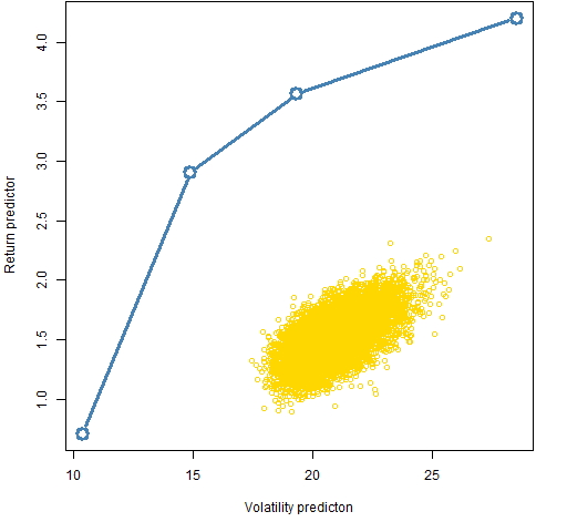

We see that the efficient frontier is seriously far from the typical random portfolio.

Realization

When we were just predicting, we were at the end of 2010.  Now we are in 2012 and we can see what actually happened in 2011.

Volatility

Figure 4 shows the quality of the volatility prediction for the random portfolios.

Figure 4: Realized volatility versus predicted volatility for the 10,000 random portfolios.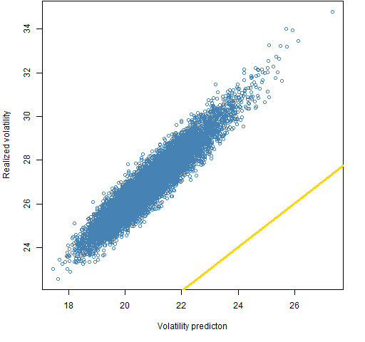

2011 turned out to be somewhat more volatile than the predictions.  The correlation among portfolios that satisfy the constraints is reasonably high.

A high correlation between predicted and realized volatility is what we need for minimum variance optimization to work.  (But this set of random portfolios doesn’t allow us to see the relationship at the extreme low end of volatility.)

Ex ante frontier

Figure 5 shows the realized version of Figure 3.

Figure 5: Realized return versus volatility of the 10,000 random portfolios, plus points on the ex-ante efficient frontier.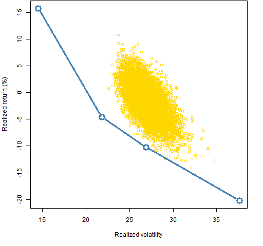

Figure 5 looks nothing like it is “supposed” to.  This appears to be an advertisement for low volatility investing, but part of what we see is that this return predictor did not work in this time period.  If the return estimate worked, then the efficient frontier would be above the random portfolio cloud rather than below it.

However, it does seem quite extraordinary that this minimum variance portfolio should return 15% in a year when the underlying index was flat.

Ex post frontier

Figure 6 adds the ex-post efficient frontier to what is in Figure 5.  This is what could have been achieved with perfect foresight — this is much more imaginary than even the ex-ante efficient frontier.

Figure 6: Realized return versus volatility of the 10,000 random portfolios, plus points on the ex-ante and ex-post efficient frontiers.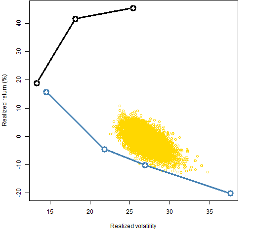

The first thing to notice is that the actual minimum variance portfolio achieved almost as small a variance as possible. The difference in returns between the two minimum variance portfolios is accidental in a sense.

The next thing to notice is that the ex-post frontier is severely truncated in terms of volatility.  The maximum return portfolio has a volatility that is smaller than 85% of the random portfolios.  This is an advertisement for low volatility investing — in retrospect for 2011.

Questions

Are there good reasons for the shape of Figure 1?

 

Appendix R

Here is a summary of the R computations that were done.

get data

The functions that downloaded the data and estimated MACD are among the functions that support the Portfolio Probe User’s Manual.  These depend on the TTR package, hence:

require(TTR)

sp5.close <- as.matrix(pp.TTR.multsymbol(sp5.names, 20060101, 20120224))

check data

There were some stocks that didn’t have the exact range of data and so consisted of all missing values.  We delete these:

sp5.close <- sp5.close[, !is.na(sp5.close[1,])]

It is good practice to inspect data for weirdness.  Our eyes are really good at that.  Here is the code I used to look through all the data series.

plot(1:4)
par(ask=TRUE)
for(i in 1:474) plot(sp5.close[,i], type='l', main=colnames(sp5.close)[i])

The initial plot command was just to get a graphics device running that could then be set to prompt for each new plot.

Nothing untoward was seen.

estimate predictors

sp5.macd <- as.matrix(pp.TTR.multmacd(sp5.close))

sp5.ret <- diff(log(sp5.close))

The variance estimation uses a function from the BurStFin package.

require(BurStFin)
sp5.var10 <- var.shrink.eqcor(sp5.ret[1006:1258, ])

generate random portfolios

The tasks done here can be done in any recent version of Portfolio Probe, but some things are easier using features new to the latest beta version.

require(PortfolioProbeBeta)

sp5.price10 <- sp5.close[1259,]
sp5.alpha10 <- sp5.macd[1259,]

rp1.sp5 <- random.portfolio(1e4, sp5.price10, sp5.var10, gross=1e6, long.only=TRUE, risk.fraction=.03, port.size=c(90,100))

random portfolio ex ante values

rp1.sp5.xa <- randport.eval(rp1.sp5, keep=c('var.values', 'alpha.values'), additional.args=list(expected.return=sp5.alpha10))

The result of the command above is a list with a component for each of the 10,000 random portfolios.  Each of those components is a list that contains the ex ante variance and expected return for the portfolio.  The command below reconfigures that into a more useful matrix.

rp1.sp5.xamat <- do.call('rbind', lapply(rp1.sp5.xa, function(x) c(volatility=sqrt(252 * x$var.values)*100, prediction=x$alpha.values)))

random portfolio ex post values

Create the matrix of closing prices during 2011:

sp5.close11 <- sp5.close[1259:1511,]

Now is when the latest beta version comes in handy — valuation now can compute returns.

rp1.sp5.xpvol <- apply(valuation(rp1.sp5, prices=sp5.close11, returns="log"), 2, sd) * sqrt(252) * 100

rp1.sp5.xpret <- 100 * valuation(rp1.sp5, prices=sp5.close11[c(1, nrow(sp5.close11)),],  returns="simple")

optimize portfolios

Here is the command to get the minimum variance portfolio.  The expected returns (sp5.alpha10) are ignored in this command except to note what the portfolio expected return is.

op1.mv.sp5 <- trade.optimizer(sp5.price10, sp5.var10, sp5.alpha10, gross=1e6, long.only=TRUE, risk.fraction=.03, port.size=c(90,100), utility="minimum variance")

Subscribe to the Portfolio Probe blog by Email