How fat tailed are returns, and how does it change over time?
Previously
The sister post of this one is “A slice of S&P 500 skewness history”.
Orientation
The word “kurtosis” is a bit weird. The original idea was of peakedness — how peaked is the distribution at the center. That’s what we can see, as in Figure 1. But it is the tail that wags the model. The modern idea of kurtosis is of fat tails (or long tails).
Figure 1: Densities of a Student’s t with 5 degrees of freedom and scaled to have variance 1 (blue), and standard normal (gold). 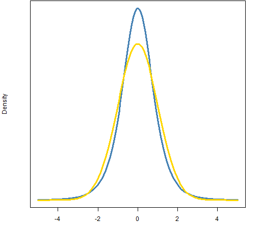 The normal distribution has a kurtosis of 3. The t-distribution in Figure 1 has a kurtosis of 9.
Sometimes “excess kurtosis” rather than kurtosis is reported. Excess kurtosis is kurtosis minus 3. So the normal distribution has excess kurtosis of 0, and Figure 1’s t has an excess kurtosis of 6. It is good to have simple ways to make things really confusing.
The data
Daily log returns of the S&P 500 from 1950 to 2011 October 17 were lying about. It is log returns (rather than simple returns) that we would expect to be normally distributed.
Kurtosis through time
Figure 2 shows rolling 250-day estimates of kurtosis on the S&P 500 daily returns.
Figure 2: Rolling kurtosis on 1-day S&P 500 returns — window is 250 observations. 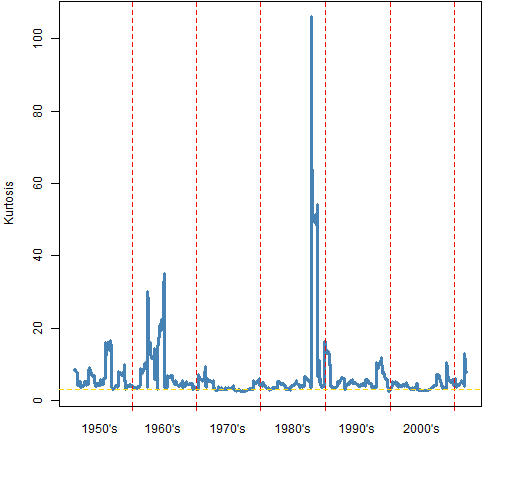
Figures 3 and 4 show rolling windows for (essentially) weekly and monthly returns. The entry and exit points of the 1987 crash is clearly visible in each of the plots. That a single data point can seriously influence the estimate means that these estimates are suspect. (This is what statistical robustness is about.)
Figure 3: Rolling kurtosis on 5-day S&P 500 returns — window is 100 observations. 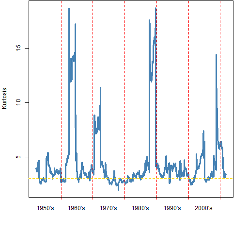
Figure 4: Rolling kurtosis on 20-day S&P 500 returns — window is 50 observations. 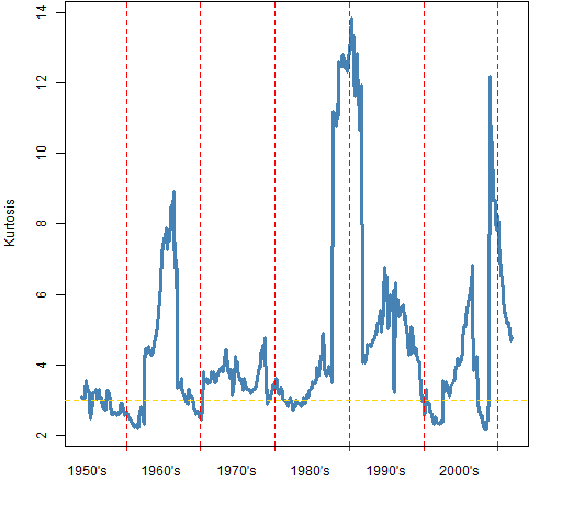
Kurtosis variability
Now instead of looking across time, we treat the data as one sample, and we can bootstrap to see the variability of the statistic. Figure 5 shows the bootstrap distribution for the daily returns.
Figure 5: Bootstrap distribution of kurtosis for daily returns of the S&P 500. 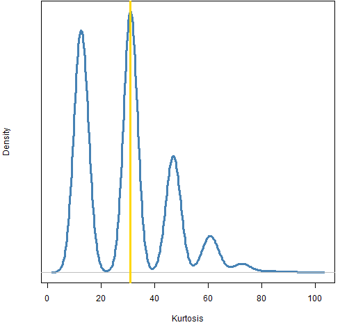 This is an interesting distribution — it has the hallmarks of a non-robust statistic with an outlier in the data. But note that the smallest of the 10,000 bootstrapped kurtosis estimates was 8.6. Even discounting the 87 crash — and numerous other events — there is a lot of kurtosis.
Figures 6, 7 and 8 show the bootstrap distributions for 5-day returns, 20-day returns and 252-day returns.
Figure 6: Bootstrap distribution of kurtosis for 5-day returns of the S&P 500. 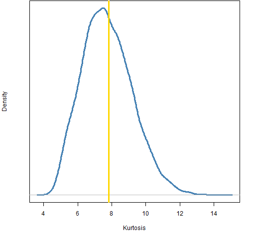
Figure 7: Bootstrap distribution of kurtosis for 20-day returns of the S&P 500. 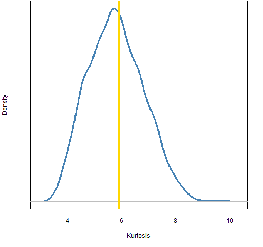
Figure 8: Bootstrap distribution of kurtosis for 252-day returns of the S&P 500. 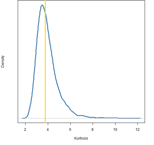
The bootstrap distributions for multiple day returns look more reasonable. We can hazard some observations based on these, but we should maintain some amount of suspicion.
Table 1: Kurtosis estimates for the S&P 500 using returns of various lengths.
| days in return |
kurtosis estimate | observations |
| 1 | 31.1 | 15,548 |
| 5 | 7.8 | 3109 |
| 20 | 5.9 | 777 |
| 252 | 3.8 | 61 |
It is clear from Table 1 that the kurtosis estimate gets smaller as the number of days in the return increases. This is evidence against the stable distribution idea. If returns did have a stable distribution, then we wouldn’t expect such a trend. In particular this seems like evidence for a finite variance.
The bootstrap distributions for 1, 5 and 20 day returns strongly argue against a normal distribution as 3 is not in their ranges.
For the 252-day returns about 11.5% of the bootstrapped kurtosis estimates are below 3. We can take this as a p-value of the null hypothesis that the kurtosis is 3 against the alternative that the kurtosis is larger than 3.
The p-value (plus Super Bowl) post gave two cases regarding beliefs and evidence in hypothesis tests. This is a third case: I inherently disbelieve the null hypothesis, but the data we have provides little evidence for rejecting it.
This case is more complicated since we need to think about how big of a difference matters — we no longer have just a binary decision. If we had more data, the p-value would undoubtedly get smaller. But with enough data it can be very small even when the true value is minutely bigger than 3.
There are undoubtedly applications where it is fine to assume that annual returns have a normal distribution. The art of modelling is to distinguish when wrong assumptions are okay to make.
Epilogue
Long tailed cat sitting by the old rocking chair
He don’t realize that there’s a danger there
from “Long Tail Cat” by Kenny Loggins
Appendix R
The functions for estimating kurtosis and skewness, and the function for aggregating daily returns are in the file aggkurtskew.R.
Update: the original version of this file had a bug in the skewness and kurtosis functions (the data were not properly centered). It was updated 2012-04-30. The numerical values in this post are off, but the patterns should be the same.
aggregate returns
Returns were aggregated like:
spxret.5d <- pp.aggsum(spxret, 5)
The pp.aggsum function already existed but didn’t do quite what was necessary for this task. (It expected a matrix, and it didn’t put names onto the result.)
It is generally very easy in R to modify an existing function to do a slightly different task.
bootstrap
The first thing to do is to create objects that will hold the bootstrapped estimates. We create several objects that are initially all the same:
bootkurt1 <- bootkurt5 <- bootkurt20 <- bootkurt252 <- numeric(1e4)
Now we do the bootstrapping:
JJl <- length(spxret)
for(i in 1:1e4) bootkurt1[i] <- pp.kurtosis(spxret[sample(JJl,JJl, replace=TRUE)])
plot(density(bootkurt1))
