Equal risk contribution of assets determines the asset weights given the variance matrix. How sensitive are those weights to the variance estimate?
Previously
The post “Risk parity” gave an overview of the idea. In particular it distinguished the cases:
- the assets have equal risk contribution
- groups of assets have equal risk contribution
A key difference is that the portfolio is fully defined by the constraint in the first case, but not in the second. This post deals with the first case (but the second case is likely to be more useful).
Shrinkage versus factors
How different are the risk parity portfolios if we estimate variance with Ledoit-Wolf shrinkage versus with a statistical factor model?
To answer that question, each type of variance was estimated on 477 constituents of the S&P 500 using daily returns. Then 200 samples of 20 assets were selected and the risk parity portfolios were formed for each selection of assets with each variance matrix. For each selection the trade distance (the value of buys plus sells divided by the portfolio value) in percent was computed.
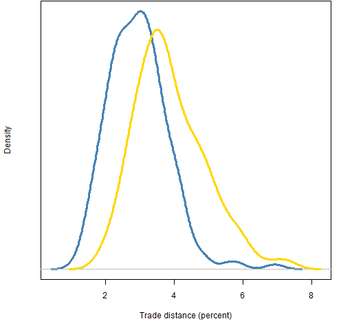
Figure 1 shows the distribution of distances when the variances are formed with returns from years 2008 or 2010.
Figure 1: Trade distance between risk parity portfolios of size 20 using factor model or Ledoit-Wolf variance estimates for years 2008 (blue) and 2010 (gold).  Interesting that the distances are smaller in 2008. I picked 2008 specifically because it was a wild ride.
The question arises: are we studying risk parity or are we studying variance estimation? A little of each I think.
Full versus specific variance estimates
The variances used to produce Figure 1 were estimated on the whole universe. The portion of those variances specific to a particular selection was then extracted for the actual computation.
An alternative is to estimate a variance matrix for each selection. So we estimate a 20 by 20 variance matrix instead of a 477 by 477 matrix.
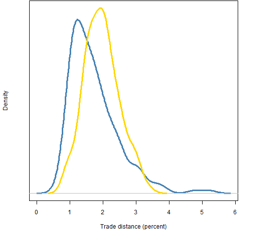
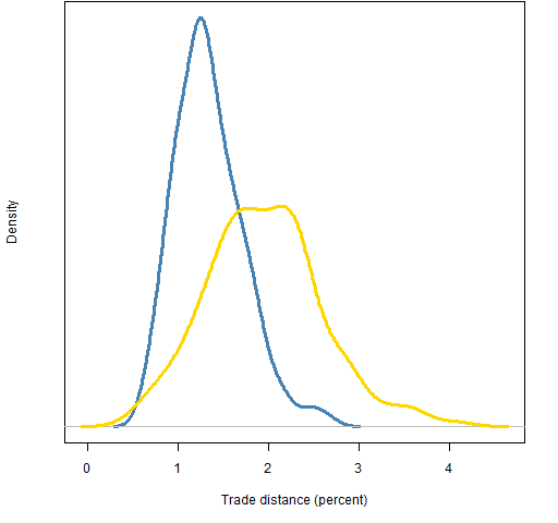
Figures 2 and 3 show the trade distances between using full versus specific estimates. It is a desirable feature to have this small.
If we were to use the sample variance, then the distance would be zero. So, good in one sense. But the sample variance is a horrible estimate for large universes. In our case of about 250 observations and 477 assets, the sample variance matrix is far from positive definite (see portfolio optimization problem 7).
Figure 2: Trade distances between risk parity portfolios of size 20 for year 2008 full versus specific variances using a factor model (blue) and Ledoit-Wolf (gold). 
This picture makes sense to me — generally the big and small factor models agree well, but occasionally there is a wide divergence.
Figure 3: Trade distances between risk parity portfolios of size 20 for year 2010 full versus specific variances using a factor model (blue) and Ledoit-Wolf (gold).  The Ledoit-Wolf distribution in 2010 is reasonably similar to that in 2008. But the distributions for factor models are quite different. Was 2008 a bad year for factor models, or was 2010 a good year?
Appendix R
variance estimation
The variance estimates use functions from the BurStFin package, available at:
install.packages("BurStFin", repos="http://www.burns-stat.com/R")
They are used like:
require(BurStFin)
varfac08 <- factor.model.stat(sp500.ret[251:503,])
varlw08 <- var.shrink.eqcor(sp500.ret[251:503,])
portfolio creation
The functions written to do this task are in the file: risk_parity_varfuns.R
Some of the data for Figure 1 was created with:
require(PortfolioProbe)
rp20dist.lwfac08 <- rep(NA, 200)
for(i in 1:200) {
rp20dist.lwfac08[i] <- pp.riskpardist(sample(sp500.id, 20))
cat(i, rp20dist.lwfac08[i], "\n")
}
The script to do all the computations is riskpartest.Rscript
missing values
The tolerance for the equality of risk was set to be quite small so that the differences between portfolios would be all due to variance differences. This meant that in a few cases a portfolio was not found that satisfied the constraints. Those cases were removed. This is an example of the strength of having missing values in the language.
A sketch for Figure 1 is created with:
plot(density(na.omit(rp20dist.lwfac08)))

Hi Pat, I was trying to load the ‘BurStFin’ package however failed with following error:
> library(BurStFin)
Error in library(BurStFin) :
package ‘BurStFin’ does not have a NAMESPACE and should be re-installed
What could be way out? I was using Windows 7 with R-2-14.0.
Thanks,
Ron,
Right, sorry. Yes, it doesn’t work in 2.14.x because it doesn’t have a namespace. That will be fixed “real soon now”.
In the weeks between now and “real soon now” perhaps the easiest way is to install it into an older version of R, ‘dump’ (or ‘save’) the functions you want, and then ‘source’ (or ‘attach’) in 2.14.x.