Do non-trading days explain the mystery of volatility estimation?
Previously
The post “The volatility mystery continues” showed that volatility estimated with daily data tends to be larger (in recent years) than when estimated with lower frequency returns.
Time adjusting
One of the comments — from Joseph Wilson — was that there is a problem with how daily returns are computed. The return for Thursday close to Friday close is over one day, but Friday close to Monday close is over three days. Joseph hypothesizes that this is the source of the bias.
His way of adjusting is to divide the usual return by the number of days. This seems like it should be too much of an adjustment — it supposes that news intensity is the same on the weekend as during trading days.
It is possible to parameterize it: divide by the number of days to some power. If the exponent is one, then it is dividing by the number of days. If the exponent is zero, no adjustment is made. An exponent between zero and one makes an intermediate adjustment.
We can test how much too big the multi-day returns are by using the one-day returns immediately surrounding them as controls. The mean of the absolute value or squares of the control returns should be equal to that of the multi-day returns.
First, we can look at how different the multi-day returns are from the controls — this is shown in Figure 1 for the S&P 500 index starting in 1989 using log returns.
Figure 1: 1-day control returns (black) compared to multi-day returns (blue). 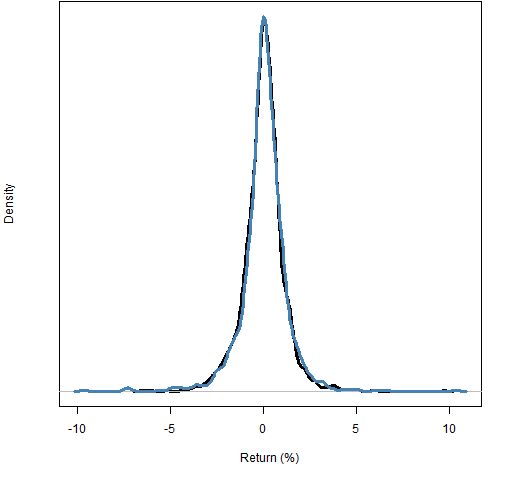 Visually, at least, there is very little difference between controls and multi-day. But we can find the exponent that makes the two equal on some measure.
Of course we can get lots of different answers by changing the question slightly. Matching absolute values we get an exponent of about 0.05; matching squares we get about 0.23.
If we throw out the 2 multi-day returns (out of 1159) that are greater than 8% in absolute value, we get exponents of 0.04 and 0.14 on the absolute and squared scales. Throwing out the 9 returns greater than 5% in absolute value, gives us exponents of 0.01 and 0.02.
So we’ve seen that the matching is very non-robust to the largest multi-day returns, and that a minimal adjustment looks to be the right thing. Figure 2 shows the distribution we get when adjusting by the largest exponent we estimated: 0.23.
Figure 2: 1-day control returns (black) compared to multi-day returns adjusted with exponent 0.23 (gold). 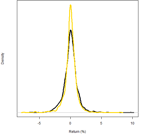 Clearly Figure 2 shows an over-adjustment.
Volatility results
Here we show the effect of (over)adjusting the returns on volatility estimation. The meaning of the plots is explained in “The volatility mystery continues”. The exponent we use to do the time adjustment is 0.23 — the largest estimate that we’ve seen.
Figure 3: Volatility estimate distributions for 20-day time-adjusted returns on block 1 (1989-01-03 to 1992-03-02). 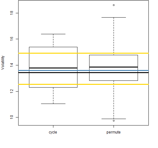
Figure 4: Volatility estimate distributions for 20-day time-adjusted returns on block 2 (1992-03-03 to 1995-05-01). 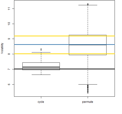
Figure 5: Volatility estimate distributions for 20-day time-adjusted returns on block 3 (1995-05-02 to 1998-06-30). 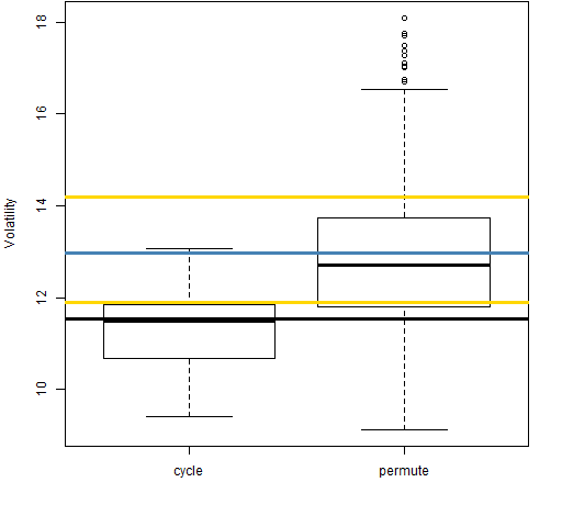
Figure 6: Volatility estimate distributions for 20-day time-adjusted returns on block 4 (1998-07-01 to 2001-08-30). 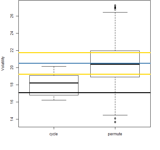
Figure 7: Volatility estimate distributions for 20-day time-adjusted returns on block 5 (2001-08-31 to 2004-11-09). 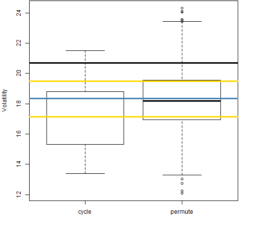
Figure 8: Volatility estimate distributions for 20-day time-adjusted returns on block 6 (2004-11-10 to 2008-01-15). 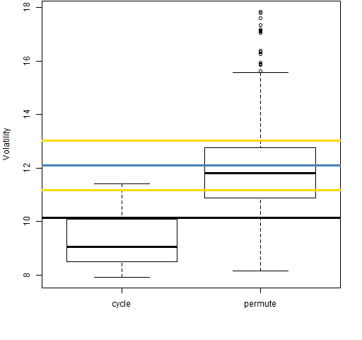
Figure 9: Volatility estimate distributions for 20-day time-adjusted returns on block 7 (2008-01-16 to 2011-03-18). 
Even with the returns over adjusted for time, the “cycle” distributions tend to be smaller than the “permute” distributions. That is, the anomaly is still there.
Summary
Hypothesis: multi-day returns cause the discrepancy between daily and monthly volatility estimates.
I found the hypothesis to be plausible. However, I think there is now sufficient evidence to rule it out.
Epilogue
Tryin’ to wipe out every trace
Of all the other days in the week
You know that this’ll be the Saturday you’re reachin’ your peak
from “(Looking for) The Heart of Saturday Night” by Tom Waits
Appendix R
Pretty much all of the analysis was done via pp.timeadj.ret and pp.tartest.
The latter function is what I think of as a fairly typical research function. It grew incoherently, is not well-structured, does too much stuff. Kludgy is the word. But it served its purpose, and if we came back to it in a year or three, we’d be able to figure out what was going on.
To get the estimated exponents, I just looked at the output of pp.tartest and guessed to the nearest hundredth. To do that automatically, you could use the uniroot function to find the actual zero.
