How do volatility estimates based on monthly versus daily returns differ?

Previously

The post “The mystery of volatility estimates from daily versus monthly returns” and its offspring “Another look at autocorrelation in the S&P 500” discussed what appears to be an anomaly in the estimation of volatility from daily versus monthly data.

In recent times estimates of volatility from monthly data appear smaller than volatility estimated from daily data.  Hypotheses about what is happening include:

• There is autocorrelation in the returns
• There is some sort of garch effect
• There is no real discrepancy, just noise

The data

The data used in the present analysis are daily log returns on the S&P 500 starting at the beginning of 1989.  This is broken into 7 blocks each of length 800 trading days — so slightly more than 3 years.  800 because it is divisible by 5 (weekly) and 20 (monthly).

The estimates for these blocks from several time scales are shown in Table 1.

Table 1: Volatility estimates with returns of different lengths (in days) for the 7 blocks.

	B1	B2	B3	B4	B5	B6	B7
1	14.4	9.1	13.9	21.4	19.6	12.5	29.7
2	14.4	9.1	13.6	20.8	19.1	11.6	29.8
5	15.1	8.4	12.0	19.2	21.5	11.2	23.9
10	14.4	7.0	11.6	19.5	21.4	9.6	23.5
20	14.4	7.2	12.0	17.2	21.9	10.4	22.5
40	15.0	6.5	9.8	15.0	15.5	10.0	27.0

The effect looks quite noisy in Table 1.  Perhaps there is nothing to investigate, but let’s persevere.

GARCH

A problem with volatility is that it is unobservable.  Using garch models can sort of help that — they give us an estimate of volatility for each time point.  Table 2 shows the results we get by averaging the garch estimates of volatility within each block.

Table 2: Volatility derived from garch models of returns of different lengths (in days) for the 7 blocks.

	B1	B2	B3	B4	B5	B6	B7
1	14.7	10.0	13.6	20.9	18.6	12.3	25.4
2	14.7	10.3	13.6	20.2	18.0	11.9	25.0
5	15.5	10.1	12.4	19.0	20.0	11.4	22.4
10	15.2	9.9	12.4	19.1	21.1	10.7	22.2
20	15.1	11.6	13.6	16.6	21.5	12.3	21.7
40	15.2	11.7	13.2	14.5	16.3	12.5	21.3

The effect looks smaller here, but there are hints that it hasn’t disappeared entirely.

If garch does explain the phenomenon (should it exist), then I would have expected how volatility acts within each block to matter.  Figure 1 shows the garch volatility, but I don’t see a connection.

Figure 1: GARCH volatility based on 1-day returns.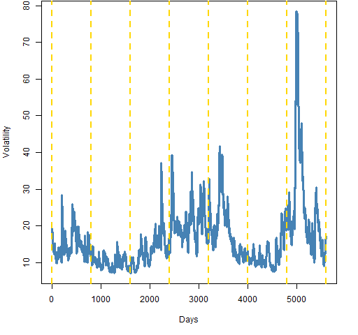

Cycles

When we aggregate the daily returns into longer time periods, the particular days that go together can matter.  Perhaps all we are seeing is that the estimates with returns from longer time frames are noisier and hence we happen to have seen small ones sometimes.

We can test this by moving the starting point through a cycle.  The way it was done here was to paste the unused values at the start onto the last data point.  So there is one artificial data point in all but one of the cycles, but the same 800 daily returns are used in each case.  We then get a distribution of volatility estimates.

We can create a different distribution which runs through the cycles but first does a random permutation of the daily returns.  With this distribution we know there is no autocorrelation.  But we are also destroying the volatility clustering, so we can’t distinguish between those two hypotheses.

The subsequent figures include:

• a boxplot of the volatility estimates from aggregations of the actual daily returns (denoted “cycle”)
• a boxplot of the volatility estimates from aggregations of permuted daily returns (denoted “permute”)
• the volatility estimate from the daily returns (horizontal blue line)
• the 95% bootstrap confidence interval of the daily volatility estimate (horizontal gold lines)
• the actual volatility estimate from aggregated data that appears in Table 1 (horizontal black line)

Figure 2: Volatility estimate distributions for 20-day returns on block 1 (1989-01-03 to 1992-03-02). 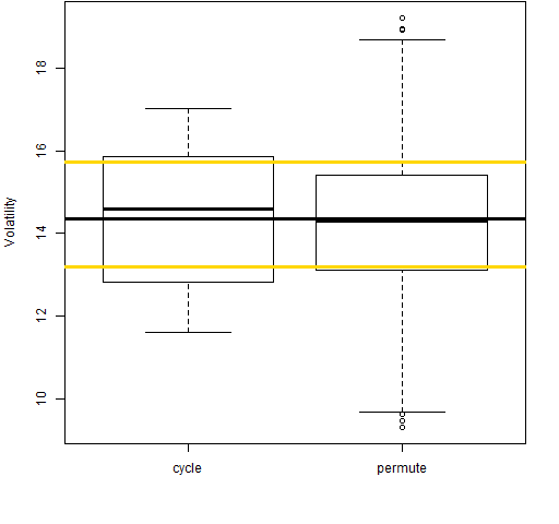In Figure 2 we see the behavior that we would expect.  Both boxplots are pretty much centered on the estimate from the daily returns.  The actual estimate from the aggregated data happens to be very close to that from the daily data, but it could have been quite far away.  This shows that the estimates with monthly data are substantially more variable than those from daily data.

Figure 3: Volatility estimate distributions for 20-day returns on block 2 (1992-03-03 to 1995-05-01). 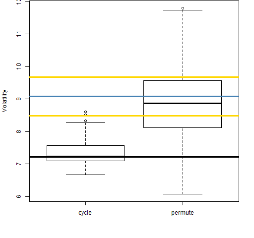In Figure 3 we see the typical pattern: the estimate from the aggregated returns is smaller than either the daily estimate or aggregation with permuted returns.

Figure 4: Volatility estimate distributions for 20-day returns on block 3 (1995-05-02 to 1998-06-30).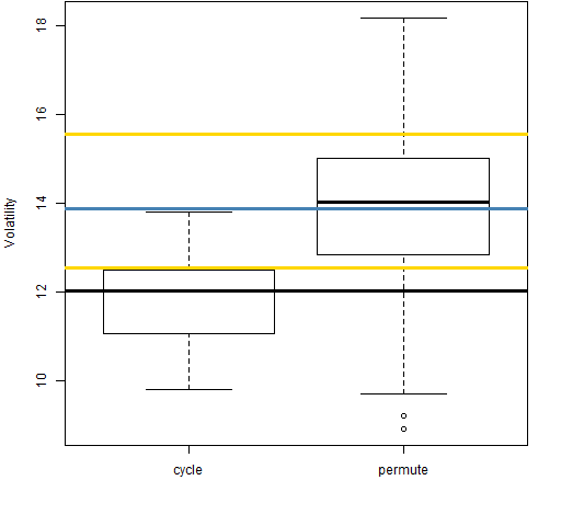

Figure 5: Volatility estimate distributions for 20-day returns on block 4 (1998-07-01 to 2001-08-30).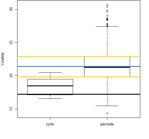

Figure 6: Volatility estimate distributions for 20-day returns on block 5 (2001-08-31 to 2004-11-09).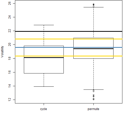

Figure 7: Volatility estimate distributions for 20-day returns on block 6 (2004-11-10 to 2008-01-15).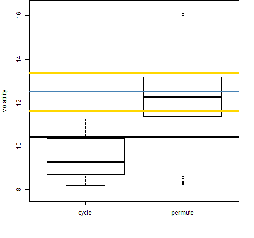

Figure 8: Volatility estimate distributions for 20-day returns on block 7 (2008-01-16 to 2011-03-18). 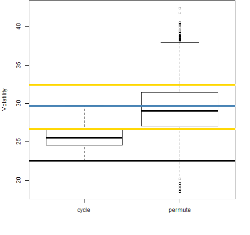Figures 2 through 8 showed the situation for aggregations to 20 days.  Figures 9 through 15 are of aggregations to 5 days.  In these cases the “cycle” boxplots are only representing 5 datapoints rather than 20.

Figure 9: Volatility estimate distributions for 5-day returns on block 1 (1989-01-03 to 1992-03-02).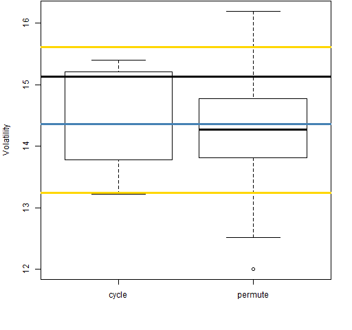

Figure 10: Volatility estimate distributions for 5-day returns on block 2 (1992-03-03 to 1995-05-01).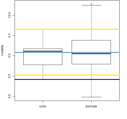

Figure 11: Volatility estimate distributions for 5-day returns on block 3 (1995-05-02 to 1998-06-30).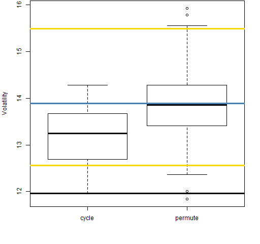

Figure 12: Volatility estimate distributions for 5-day returns on block 4 (1998-07-01 to 2001-08-30).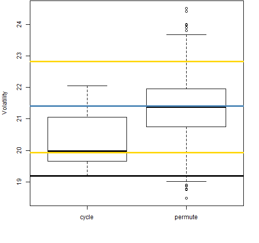

Figure 13: Volatility estimate distributions for 5-day returns on block 5 (2001-08-31 to 2004-11-09).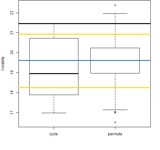

Figure 14: Volatility estimate distributions for 5-day returns on block 6 (2004-11-10 to 2008-01-15).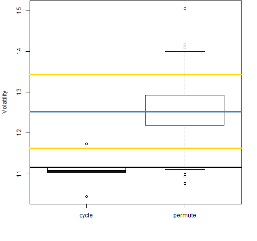

Figure 15: Volatility estimate distributions for 5-day returns on block 7 (2008-01-16 to 2011-03-18). 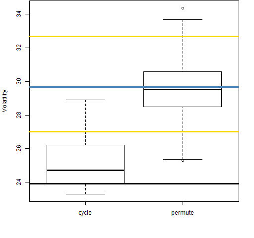There seems to be an anomaly within the anomaly in that the 40-day aggregation for block 7 displays “good” behavior as shown in Figure 16.

Figure 16: Volatility estimate distributions for 40-day returns on block 7 (2008-01-16 to 2011-03-18).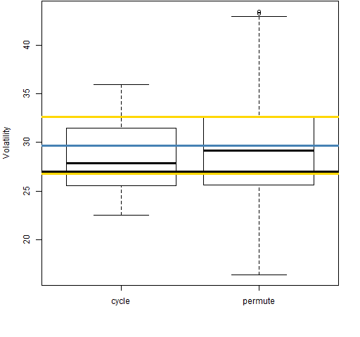

Summary

I think what’s been shown here is that there really is a phenomenon to explain.  But we haven’t yet pinned down an explanation.

There is the hypothesis that infinite variance could be the cause of the weird behavior.  I don’t believe that the variance is infinite; but if it were, I don’t think that would cause what we’ve seen here as the variance would be infinite in all cases.

Questions

How do we test if volatility clustering is causing the effect?

Epilogue

And something is happening here
But you don’t know what it is
Do you, Mister Jones ?

from “Ballad of a Thin Man” by Bob Dylan

Appendix R

There are two main parts to this analysis:

• garch estimation
• cycling, permuting and bootstrapping

garch estimation

The garch models were estimated like:

require(rugarch)
gs1t <- ugarchfit(ugarchspec(distribution='std'), spxretd1)

This estimates a garch(1,1) model assuming the residuals have a Student’s t distribution.  It also assumes an ARMA(1,1) process for the mean.  The exact specification seems to make essentially no difference for our purposes. Since we are only interested in the in-sample volatility, pretty much any semi-reasonable garch coefficients would probably do.

A basic version of Figure 1 is:

plot(sigma(gs1t) * 100 * sqrt(252), type='l')

The estimation of garch models is a surprisingly tough task.  I’ll not recommend any garch software without thoroughly investigating it.  But getting similar garch coefficients whether the returns are in their natural scale or in percent is comforting.

cycling, permuting and bootstrapping

Some functions were written to do these tasks, and are listed (with rather bizarre formatting) in volatility_est_funs.R.

paste and cut and paste

A labor-saving device to put the dates of the blocks into the figure captions was to paste (in the R sense) the dates together into strings, and then to cut and paste (in the GUI sense) those into the captions.  The R code was:

jjb <- seq(1, by=800, length=7)

paste(' (', names(spxretd1)[jjb], ' to ', names(spxretd1[jjb+799]), ')', sep='')

Subscribe to the Portfolio Probe blog by Email