How does the effect of our expected returns change over time?  This is not academic  curiosity, we want to know in the context of our portfolio if we can.  And we can — we visualize the effect of expected returns in situ.

First step

The idea is to look at the returns of portfolios that have the constraints we want and also have a high expected return.  Each of those is paired with a portfolio that  has the portfolio constraints but no constraint on expected return.  That is, we generate two sets of random portfolios and subtract the returns of one set from the other.

Figure 1 shows a distribution of realized alpha.  We are used to thinking of the effect of alpha as a number.  However, many assumptions need to be made in order to get to one number.  Those assumptions can have a big effect as witnessed by the width of the distribution in Figure 1 (but see the “fine print” section below).

Figure 1: Realized alpha of week 1 of 2007 Q2 of long-only portfolio.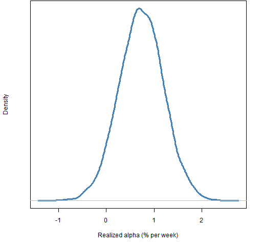

What are we doing?  We are looking at the return of a portfolio that we might hold when using our expected returns and subtracting the return from another portfolio we might hold except we ignore the expected returns when we form it.  Then we do that 9999 times again.  You may be concerned that the control portfolio is very arbitrary — we could end up with a very good one or a very bad one.  Absolutely true, but that doesn’t affect the distribution (I looked).  In particular the tails are very stable — the center peak wiggles around slightly.

To be clear, realized alpha means: the return over a given period of time of a portfolio with large expected return minus the return over the same period of a portfolio with random expected return.

The data

The data are of almost all of the constituents of the S&P 500.  The expected return is the default result from the MACD function of the TTR package in R.

The constraints used in the long-only portfolios are:

• long-only
• 45 to 50 names in the portfolio
• no asset with more than 5% weight (when the portfolio is formed)
• the sum of the 10 largest weights no more than 30%

Time decay

Figure 1 shows us just one time period.  We can enhance that by adding later time frames.  Figure 2 shows the realized alpha distributions for weeks 2 through 4, and weeks 5 through 13 as well as that for week 1.  At this point in time at least, the decay is quite slow.

Figure 2: Realized long-only alpha distribution in 2007 Q2 for: week 1 (blue), weeks 2 through 4 (gold), and weeks 5 through 13 (black).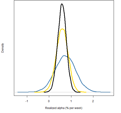

Long-short portfolios

This game can, of course, be played with long-short portfolios as well.  The constraints we use in this case are:

• net value is 10% of the gross
• 45 to 50 names in the portfolio
• no asset with more than 5% weight
• the sum of the 10 largest weights no more than 30%

The constraint on the net value was selected to try to counteract the idea that all long-short portfolios are dollar neutral.  Weights — as used here — sum in absolute value to 1.

Figure 3: Realized long-short alpha distribution in 2007 Q2 for: week 1 (blue), weeks 2 through 4 (gold), and weeks 5 through 13 (black).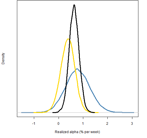

Comparing Figures 2 and 3 we can hypothesize that shorting is not helping us.  We can investigate by generating short-only portfolios that are similar to the short portion of our long-short portfolios.  The constraints are:

• long value is zero
• number of names is 18 to 22
• no asset with weight greater than 8%
• the sum of the largest 5 weights is no more than 30%

Figure 4: Realized short-only alpha distribution in 2007 Q2 for: week 1 (blue), weeks 2 through 4 (gold), and weeks 5 through 13 (black). 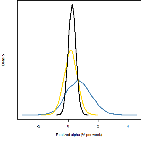While the shorts have about the same mean return as the longs for week 1, the alpha mostly decays for the later periods.

Large print

We should not think that we know something about any market process by looking at just one point in time.  I was expecting the effect of MACD to dissipate quite quickly — I’m surprised that it seems to be basically constant over a quarter.  It would take examination over several time points to understand the typical decay.

There are periods of time when MACD gives negative alpha.  It is of interest to learn the speed of decay in periods of negative alpha as well.

Also, of course, you want to select time frames that are appropriate for the strategy that you have.  It looks as though we probably want to look at periods much longer than a quarter for MACD, for instance.

Fine print

So far I’ve glossed over the bound on the alpha constraint.

Figures 1 and 2 constrain alpha to be at least 4.5 when the maximum possible alpha given the other constraints is about 5.07.  Figures 5, 6 and 7 compare the return distributions (no subtraction of controls) of using the 4.5 bound versus increasing that to 5.

Figure 5: Return distribution for long-only portfolios during week 1 of 2007 Q2 with alpha at least 4.5 (blue) or at least 5 (gold). 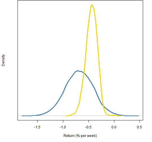Figure 6: Return distribution for long-only portfolios during weeks 2 through 4 of 2007 Q2 with alpha at least 4.5 (blue) or at least 5 (gold).

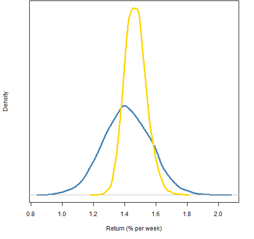
Figure 7: Return distribution for long-only portfolios during weeks 5 through 13 of 2007 Q2 with alpha at least 4.5 (blue) or at least 5 (gold).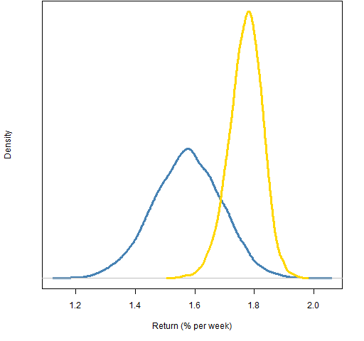

From these figures we can see that the bound has a definite effect.

You might initially think that the tighter the bound the better.  There’s a practical issue that you might wait a long time if you try a very tight constraint.  But a tight constraint might not be appropriate in the first place.  When you actually have a portfolio, you have turnover constraints of some form.  That means that you are probably constrained from getting close to the absolutely best alpha.

One idea of how to select the alpha bound would be to use a given percentile of the distribution of asset alphas.  For instance use the 90th percentile of the alpha distribution at each point in time.

A refinement on that idea would be to find the percentile of the maximum alpha portfolio at each point and then back off a certain amount.  For example if our back-off amount is 5 percentiles, then a maximum alpha at the 97th percentile of the alpha distribution would mean our alpha bound would be at the 92nd percentile but a maximum alpha at the 93rd percentile would mean our bound would be at the 88th percentile.

Appendix R

There are just three simple steps to do this sort of analysis:

• generate random portfolios
• compute the returns
• plot the results

The long-only analysis is quite trivial, but there are a couple of tricky bits in long-short land so we’ll focus attention there.

generate random portfolios

require(PortfolioProbe)

rpls.39.a4 <- random.portfolio(1e4, prices=sp500.closeok[39,], expected.return=sp500.macd[39,], gross=1e6, net=1e5, port.size=c(45,50), max.weight=.05, sum.weight=c('10'=.3), alpha.constraint=4)

The other set of random portfolios are computed the same way except the alpha constraint is removed.

compute the returns

retls.39.wk2to4 <- pp.simpret(valuation(rpls.39, sp500.closeok[c(44, 59),], collapse=TRUE, type="nav", cash=9e5))

The command above is one of the tricky bits.  How do you compute returns for a long-short portfolio?

In the long-only case we start with one million dollars in our hand.  We then use all of it to buy shares; now we have zero cash but the net value of our portfolio is one million.

In the long-short case we start with one million dollars.  We use 550 thousand to buy shares, so we have 450 thousand left in cash; now we sell 450 thousand short, so we get another 450 thousand in cash.  We now have 900 thousand in cash and the net value of our portfolio is 100 thousand.

The return is computed from the net asset value at the start and end times.

There’s another tricky bit with the short-only portfolios.  In terms of returns going short reverses time, so here we reverse time in the prices matrix:

retso.39.wk2to4.a3 <- pp.simpret(valuation(rpso.39.a3, sp500.closeok[c(59, 44),], collapse=TRUE))

plot the results

This merely involves using the density function, and then using xlim and ylim arguments to plot in order to be able to see everything.

Subscribe to the Portfolio Probe blog by Email