What drives the estimates apart?
Previously
A post by Investment Performance Guy prompted “Variability of volatility estimates from daily data”.
In my comments to the original post I suggested that using daily data to estimate volatility would be equivalent to using monthly data except with less variability. Dave, the Investment Performance Guy, proposed the exquisitely reasonable next step: prove it. (But he phrased it much more politely.)
Data
Daily closing log returns of the S&P 500 from the start of 1950.
Three-year non-overlapping periods were used. So the estimates with monthly data use 36 data points, and the daily estimates use about 756 data points.
The monthly estimates are annualized by multiplying the standard deviation by the square root of 12. The daily estimates are annualized with the square root of 252.
Differences
Figure 1 shows what I expected to get when comparing the difference between the estimates of volatility (annualized standard deviation in percent) using daily or monthly data. The line wiggles around zero.
Figure 1: The daily volatility estimate minus the monthly estimate for each three-year period starting in 1950 through 1997. 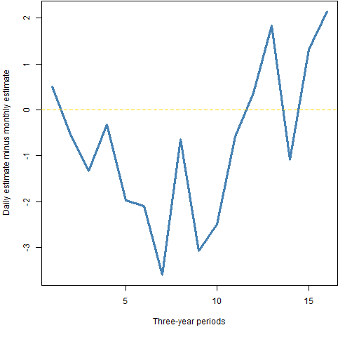 Figure 2 shows the full results, and we get a different impression. In case you didn’t think it before from Figure 1, the run of 10 estimates where daily is less than monthly is fairly extraordinary if they were estimating the same thing.
Figure 2: The daily volatility estimate minus the monthly estimate for each three-year period starting in 1950. 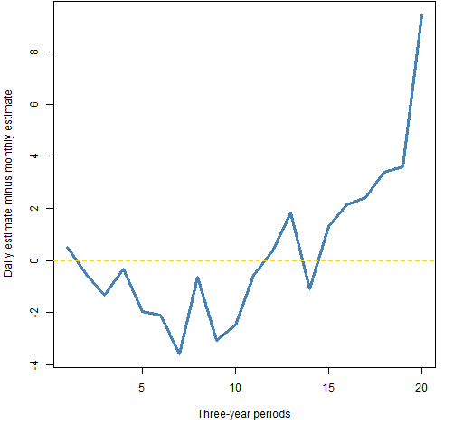 Figure 3 moves the windows over by one year. We get a similar pattern to that in Figure 2.
Figure 3: The daily volatility estimate minus the monthly estimate for each three-year period starting in 1951. 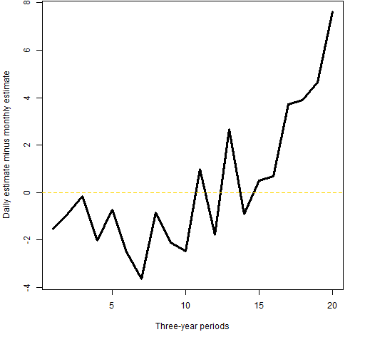
The New York Times had a recent piece on “excess volatility” that echoes the results here. (Note, though, that “excess volatility” is often used in a different sense.)
Figure 4 shows the monthly versus daily estimates for the three-year periods along with 95% bootstrap confidence intervals.
Figure 4: Point estimates and 95% confidence intervals for monthly and daily volatility estimates on three-year periods starting in 1950. 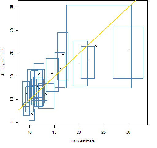 The right-most box is for years 2007-2009. The gigantic box is years 1986-1988 — it is gigantic because there is a data point that is about -23% (daily) or -25% (monthly) which can appear numerous times in a bootstrap sample, or not at all. The small box that sticks out at the bottom is 2004-2006.
The ratio of the heights of the boxes to their widths shows the advantage of using daily versus monthly data in terms of variability of the estimate.
Autocorrelation
If the data obeyed the assumptions that statisticians want to have, then the monthly and daily estimates would be giving us the same thing up to estimation error. The above figures suggest that perhaps they aren’t aiming at the same place — that is, that there’s an assumption that fails.
My original point of view that prompted this post was not that the assumptions held, but that they wouldn’t fail by enough to make a material difference. I seem to have been wrong.
What we are seeing seems to imply that the S&P random walk is falling off the tightrope — that there is autocorrelation of some sort in the data.
Figure 5 shows the estimate from an AR(1) model on running windows of 250 trading days. The yellow lines are the 95% confidence interval for randomly sampled daily returns. The width of true confidence intervals will vary over time, but this gives a rough idea.
Figure 5: autoregression coefficient on running 250-day windows. 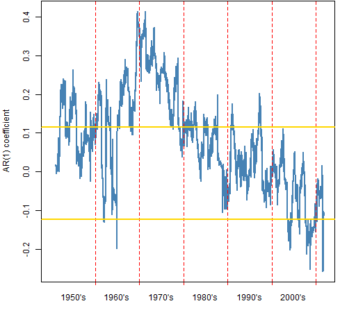 Positive autocorrelation implies momentum and that the monthly volatility estimates would tend to be larger than the daily estimates. Negative autocorrelation implies mean reversion and that the daily estimates would tend to be larger than the monthly estimates.
The positive autocorrelation in decades past might have been due to stale prices, and hence not a money-making opportunity. However, if that were the case, I would expect it to have been more consistently positive from the start of the data.
The AR(1) model need not be an especially good reflection of the time dependency that is in the returns. And it probably isn’t.
Figure 6 compares the volatility estimates over time.
Figure 6: Monthly (blue) and daily (black) volatility estimates over each three-year period starting in 1950. 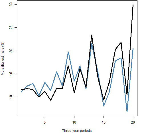
Questions
Is the presumed mean reversion in the market lately a good thing or a bad thing?
Why would it be there?
Is there a way to “properly” annualize volatility?
What is the connection between what we’ve just seen and “Is momentum really momentum?” by Robert Novy-Marx (which comes to us via Whitebox Selected Research)?
Appendix R
The computations and graphs were (of course) done in R.
daily to monthly
The daily returns are just a vector with names in the form of "1950-01-04". The command to get monthly returns was:
spxmonret <- tapply(spxret, substring(names(spxret),1,7), sum)
This categorizes each observation by month and sums the elements within each month.
bespoke functions
The function that does all the work (estimates and confidence intervals) is pp.volcompare.
Figure 4 was created with the aid of function pp.plot2ci and Figure 5 used pp.timeplot.
autoregression estimation
The data for Figure 5 was computed with:
spx.ar1 <- spxret
spx.ar1[] <- NA
for(i in 250:length(spxret)) spx.ar1[i] <- ar(spxret[seq(to=i, length=250)], order=1, aic=FALSE)$ar
spx.ar1boot <- numeric(1e4)
for(i in 1:1e4) spx.ar1boot[i] <- ar(spxret[sample(15548, 250)], order=1, aic=FALSE)$ar
A simplified version of the command to add the confidence interval to the plot is:
abline(h=quantile(spx.ar1boot, c(.025, .975)))
Pat, I’d like to offer some comments, since S&P500 volatility modeling has been explored to death, and with good empirical results. You are taking as null hypothesis the independent, identically distributed lognormal returns, and then relax the notion of independence by inferring (from the ACF and AR(1)) that there is some kind of serial dependence in returns. However, you have to keep in mind that the estimates of an AR model, the confidence intervals corresponding to the null of uncorrelated returns etc. depend crucially on i) normality of returns; ii) stationarity. Definitely i) is not satisfied, since returns are heavy tailed; ii) may be, but on short intervals, and am not sure that 252 days is short enough.
Autocorrelation tests are often misleading because users often apply them automatically without examining the assumptions. For example, you may have positive/negative autocorrelation even if returns are iid and lognormal, but you have a stochastic (unobservable) drift. For example, from a statistical perspective, the momentum anomaly relies on non-zero expected returns, definitely not on positive short-term autocorrelation of stock returns. It is an unwarranted if common assumption to think that existence of momentum or mean reversion imply asset-level serial dependence.
It is sufficient to assume non-normal (unconditional) returns to explain the difference between monthly and daily estimates of annualized volatility. If you assume conditionally normal returns with stochastic volatility you have GARCH models; if the conditional returns are heavy-tailed, you have Levy process. Dozens of papers have been written of either family, but all explain stylized facts about predicted volatility at different time horizons.
Gappy, thanks for your comments.
I agree that the confidence interval on the AR model is suspect, but it is not suspect because of non-normality. The confidence interval is from a bootstrap so the distributional assumption is avoided.
There has been a change over the decades of whether it is monthly or daily estimates that are bigger. So it seems to me that there is not going to be any one tweak in assumptions that is going to explain everything.
OK, I checked the way you estimated the confidence interval. I would not proceed this way. You are assuming that the SPX returns are drawn from the same distribution throughout the entire available history, and are sampling without replacement. In the code linked below, I sample with replacement in non-overlapping blocks of one year, and I perform a multiple test of hypothesis with Bonferroni correction. The one year is motivated by the assumption that reutrns are approximately stationary in this interval, and the nonoverlapping blocks are motivated by the need to perform independent tests. From this test, you can see that definitely SPX would reject the null if the mid 60’s-mid 70’s are included, but is not rejected using the last 30 years of returns.
To give tentative answers to your three questions:
1) non sure in mean reversion is “good” or “bad”. I would just stress the adjective “presumed”;
2) why *was* it there40+ years ago? What has changed?
3) rather than focus on AR models, I would try a GARCH model. I don’t used them regularly, but have read that EGARCH (Nelson, ‘Conditional heteroskedasticity in asset returns: A new approach’, Econometrica 1991) is parsimonious and should help explain the monthly/daily estimates discrepancy.
http://sites.google.com/site/gappy3000/filecab/spxanalysis.R
Gappy, Well done. I’ve shown your plot with some comment in a new post: https://www.portfolioprobe.com/2011/11/11/another-look-at-autocorrelation-in-the-sp-500/
Hi, I am new to this science and I have a question (which is rather naive I guess). You mentioned in your post that ‘Positive autocorrelation implies momentum and that the monthly volatility estimates would tend to be larger than the daily estimates’. I don’t understand how the positive autocorrelation is linked to the fact that monthly volatility estimated tend to be larger than the daily estimates.
Thank you.
Beth,
Think about it if we had close to perfect autocorrelation. If the autocorrelation is close to 1 and the first daily return is positive, then all the daily returns will be positive. So the month will have a large return. If the autocorrelation is close to -1, then the signs of the daily returns will tend to alternate and the monthly return will be close to zero.
Now I got it! Thank you so much!!!
Well, the post is old but only now have I managed to find it.
First of all thank you for tackling the direct question, even though in practice one finds it very often, the answers remain very obscure to me and people seldom focus on this specific topic.
Now, I’m not trying to be lazy, but is there no way to simply answer question number 3? I mean, the GARCH procedure seems a bit complicated just to measure volatility from historical prices.
Thanks!!!
pablete,
I suspect that simple is good enough for almost all uses. A closer-to-perfect annualization is unlikely to have much effect, and putting your efforts into making sure you have the big picture right is probably a better use of resources.
But, of course, I’m open to ideas about better methods.
Pingback: Blog year 2012 in review | Portfolio Probe | Generate random portfolios. Fund management software by Burns Statistics
Pingback: Another look at autocorrelation in the S&P 500 | Portfolio Probe | Generate random portfolios. Fund management software by Burns Statistics
Pingback: The volatility mystery continues | Portfolio Probe | Generate random portfolios. Fund management software by Burns Statistics
Pingback: Volatility from daily or monthly: garch evidence | Portfolio Probe | Generate random portfolios. Fund management software by Burns Statistics
Pingback: Popular posts 2013 October | Portfolio Probe | Generate random portfolios. Fund management software by Burns Statistics
Pingback: Blog year 2013 in review | Portfolio Probe | Generate random portfolios. Fund management software by Burns Statistics
Dear Sirs,
I was having this same discussion with a friend some days ago… I would appreciate if you could conclude what would you consider more appropiate for measuring a Fund Volatility against the S&P in a period of time, the monthly or the daily volatility…
regards
T
Pat/gappy,
I am analyzing several different stock indexes am seeing a similar phenomenon — the monthly volatility is coming out much lower than the daily volatility multiplied by sqrt(days_in_a_month) implying (on average) some kind of intra-month mean reversion versus iid return series.
Would you know of a paper I could reference that corroborates/documents this empirical result? I don’t really care about stochastic models (although it is fine if the are in there), just some kind of documentation of this result.
Thanks!
Matt
Proof: Assume you have an asset that has daily returns of: +100%, -50%, 100%, -50%, etc. Your monthly returns will be 0% and your monthly SD will 0. Measuring annual volatility from daily returns will not get you an annualized volatility of 0.