It is ever so easy to make blunders when doing quantitative finance. Very popular with novices is to analyze prices rather than returns.
Regression on the prices
When you want returns, you should understand log returns versus simple returns. Here we will be randomly generating our “returns” (with R) and we will act as if they are log returns.
We generate 250 random numbers from a Student’s t distribution with 6 degrees of freedom:
> ret1 <- rt(250, 6) / 100
So we are imitating about one year’s worth of daily data. Then we can create a price series out of the returns and plot the prices:
> price1 <- 10 * exp(cumsum(ret1))
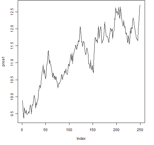
> plot(price1, type='l') # Figure 1
Figure 1: The randomly generated price series. Let’s make the novice mistake and perform a linear regression to get the trend for the prices:
> seq1 <- 1:250
> summary(lm(price1 ~ seq1)) # the novice mistake
Call:
lm(formula = price1 ~ seq1)
Residuals:
Min 1Q Median 3Q Max
-0.79084 -0.29531 0.00158 0.28625 0.91303
Coefficients:
Estimate Std. Error t value Pr(>|t|)
(Intercept) 9.8615883 0.0462913 213.03 <2e-16 ***
seq1 0.0105576 0.0003198 33.02 <2e-16 ***
---
Signif. codes: 0 ‘***’ 0.001 ‘**’ 0.01 ‘*’ 0.05 ‘.’ 0.1 ‘ ’ 1
Residual standard error: 0.3649 on 248 degrees of freedom
Multiple R-squared: 0.8147, Adjusted R-squared: 0.8139
F-statistic: 1090 on 1 and 248 DF, p-value: < 2.2e-16
Note that the coefficient for seq1 (the trend) is highly significant, as is (equivalently in this case) the overall regression.
Bootstrapping the regression
We can use the statistical bootstrap to see the variability of the trend coefficient.
> bootco1 <- numeric(1000)
> for(i in 1:1000) {
+ bsamp <- sample(250, 250, replace=TRUE)
+ bootco1[i] <- coef(lm(price1[bsamp] ~
+ seq1[bsamp]))[2]
+ }
> quantile(bootco1, c(.025, .975))
2.5% 97.5%
0.009885522 0.011224954
So the trend coefficient is very close to 0.01.
Multiple price regressions
We’ve looked at one example. Let’s do the same thing several times to get a real feel for what is going on.
We could create more objects like price1, but the “R way” of doing this is to create a list where each component is like price1.
> rlist <- vector("list", 5)
> for(i in 1:5) rlist[[i]] <- rt(250, 6) / 100
> plist <- lapply(rlist, function(x) 10 * exp(cumsum(x)))
Above we have created 5 return vectors in a list, and then created a new list holding the 5 corresponding price vectors.
Now we bootstrap the trend coefficient for each price series:
> blist <- rep(list(numeric(1000)), 5)
> for(j in 1:1000) {
+ bsamp <- sample(250, 250, replace=TRUE)
+ for(i in 1:5) {
+ blist[[i]][j] <- coef(lm(plist[[i]][bsamp]
+ ~ seq1[bsamp]))[2]
+ }
+ }
A plot of the bootstrap distributions is then made:
> dlist <- lapply(blist, density)
> dx.range <- range(lapply(dlist, "[", "x"))
> dy.range <- range(lapply(dlist, "[", "y"))
> plot(0, 0, type="n", xlim=dx.range, ylim=dy.range,
+ xlab="Coefficient value", ylab="Density")
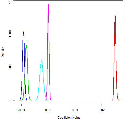
> for(i in 1:5) lines(dlist[[i]], col=i+1, lwd=2)
Figure 2: Bootstrap distributions of price trend coefficients.
So we have used the exact same random generation method for five datasets and we get significantly different results from them. Something has to be wrong.
But why?
In The tightrope of the random walk I imply that if a price series is a random walk, then the returns are uncorrelated. That is, the returns are very much like a random sample.
The reality is that prices don’t exactly follow a random walk. But they will be close enough that treating returns as uncorrelated is unlikely to lead you astray.
But prices (of the same asset across time) are correlated. Very correlated. If halfway through the year the price is higher than the starting price, then it is likely the final price of the year will be higher as well — even when there is no trend.
Variance
If we want a variance matrix, then we should also do our computation on returns and not prices.
Each of the five series that we generated were independent of each other, so they should be uncorrelated. Here’s the variance we get for the price series:
> round(var(do.call("cbind", plist)), 2)
[,1] [,2] [,3] [,4] [,5]
[1,] 3.56 -1.17 -1.26 -0.39 -0.05
[2,] -1.17 0.68 0.41 0.38 0.14
[3,] -1.26 0.41 0.59 0.20 0.01
[4,] -0.39 0.38 0.20 0.43 0.13
[5,] -0.05 0.14 0.01 0.13 0.14
Alternatively we can compute the correlation matrix for the prices:
> round(cor(do.call("cbind", plist)), 3)
[,1] [,2] [,3] [,4] [,5]
[1,] 1.000 -0.753 -0.868 -0.311 -0.067
[2,] -0.753 1.000 0.649 0.705 0.460
[3,] -0.868 0.649 1.000 0.393 0.026
[4,] -0.311 0.705 0.393 1.000 0.511
[5,] -0.067 0.460 0.026 0.511 1.000
Here is the variance for the returns (in percent):
> round(var(do.call("cbind", rlist))*1e4, 2)
[,1] [,2] [,3] [,4] [,5]
[1,] 1.48 0.03 0.06 0.05 -0.04
[2,] 0.03 1.57 -0.06 0.20 0.03
[3,] 0.06 -0.06 1.80 -0.09 0.09
[4,] 0.05 0.20 -0.09 1.52 0.06
[5,] -0.04 0.03 0.09 0.06 1.42
This looks more like what we should expect: the diagonal elements are all very similar and the off-diagonal elements are reasonably close to zero.
Epilogue
Photo by H. Dickins via everystockphoto.com.


I’m not altogether clear on what you are trying to demonstrate with your first example, how should one find the trend if not with the price?
Craig,
Thanks for your question.
If you look at Figure 2, you see that for that sample of 5 series one trend is decidedly positive, 3 are negative and one is about zero. Since they were all generated the same way, this can’t be a reasonable definition of “trend”.
The real way to look for the trend is to look at the mean return.
The returns were generated to have mean zero. So there is not a real trend in any of the price series. But any given price series will likely be reasonably up at the end of the year or down at the end of the year.
The key thing is that returns (for non-overlapping time periods) are essentially independent observations, but prices are not.
Thank you, that makes sense.
There are still times when we regress prices however, for example, when determining hedge ratios for pairs trades.
Sounds to me like you are assuming cointegration there.
This is great stuff! Please more R based posts. Thanks!
We know that regressions on prices are useless and regressions on returns are the way to go. Are you OK with regressions on log prices? See Pairs Trading Quantitative Methods and Analysis by Vidyamurthy where he performs these regressions and then looks to model the residual as mean reverting for trade signaling. I guess this is OK as in the end it is the difference of these log(prices) which is essentially the return that is being used.
I don’t know that work, so I can’t comment specifically.
The thing to ask yourself is: Are you using one realization, or are you using a lot of (almost) independent observations?
But, given Uwe’s Maxim (computers are cheap and thinking hurts), another approach is to simulate some data and see if the method gives you reasonable results. An approach I took in the post.
It looks cool! Why did you choose 10*exp(cumsum(x)) as the random function?
Matt, that’s a good question, but let’s back up one line:
ret1 <- rt(250, 6) / 100 Dividing by 100 gives a reasonable level of volatility assuming daily returns. If you want higher volatility, then divide by something smaller; and vice versa. price1 <- 10 * exp(cumsum(ret1)) The 10 is the approximate initial price. If you wanted the first price to be exactly 10, then you would do: price1 <- 10 * exp(c(0, cumsum(ret1))) Using 'cumsum' allows you to get each of the log returns from the start in the whole series -- see "A tale of two returns" for more details.
Pingback: Quantitative thoughts » Interesting volatility measurement, part 2
I am not sure if your point is that – the price is random walk but if we use prices as oppose to returns we get a significant trend. Most of the time we do not look for an explanation for the price moves but for a model to gain from. So you can force this coefficient to zero in your modelling and ignore it alltogether, and in any case, it is not siginifcantly zero but the effect is very small for this specific realiztion. and might vanish completely for a price level of e.g. 30. My point is I am not sure its enough to decide -> Return.. not levels, using this sole argument.
Eran,
Whether prices follow a random walk or not is not the issue — what matters is that there is dependence between prices at different times.
You need to ask yourself: Is the statistical technique I’m using assuming that the observations are independently distributed?
If the answer is “yes”, then you need to use returns and not prices. Techniques in this category include regression, standard error of the mean, …
If the answer is “no”, then you are free to use prices. Techniques in this category include some smoothers, seasonal decomposition, …
hmm….regression does not assume that observations are id, only the error terms should be iid. Think about simple linear regression of some measured linear relationship, how could the obervations possibly be independant?
Mor,
Yes, I could have been more clear with that statement. Thanks.
But doesn’t that mean that the question exactly is whether or not there is a unitroot not simply whether there is dependence?
Hello,
I am a little late to the party, but just getting started with proper statistical analysis of financial data.
After reading the post and the comments, I understand the main idea as such: even with a random white noise, there can be false indicators of trends in price. Returns are significantly immune to these false biases.
In your reply above, as you state, if the statistical method assumes residues are independently distributed, then we should use returns for modelling/predictions.
But what if:
1) we know that residues are not pure Gaussian IID process? Can we still go ahead with price model, and then use the *residues* from the model (which still are correlated) for other techniques on non-stationary data.
OR
2) fractionally differentiated time series? There, we can achieve stationarity but still maintain some memory, in the fractionally differenced series. We don’t have independent distribution, but shouldn’t retaining the memory help us better model the time series? Maybe fractional differentiation better helps to separate IID noise from true correlations in price?
My perception of what quants try to do was: study underlying correlations in a time series from the past, to bet on it in the future. But it seems that correlations in prices is not reliable. One should look for correlations in returns, because correlation in prices is a false positive, where even if the underlying statistical process was white noise, we end up with false trends.
Thank you for the post. I have been trying all sorts of combinations, and was never sure if I should model on price or returns or some other combination (returns time volume or whatever).
Jesper,
We imply that we accept there is a unit root in prices when we accept returns as useful in this context. But I don’t think there needs to be a unit root for data not to be useful. Agree or not?
Well first of all you’re example is very instructive so thank you for the example and for the quick reply.
I guess one argument for using first differences is the unit root hypothesis. Also S.J. Taylor argued that “prices have high correlation and because of that are hard to work with”.
When reading you’re reply to Eran:
“Eran,
Whether prices follow a random walk or not is not the issue — what matters is that there is dependence between prices at different times.”
I guess I was focusing to much on the above quote – stating only dependence – not taking into consideration what you also said:
“The reality is that prices don’t exactly follow a random walk. But they will be close enough that treating returns as uncorrelated is unlikely to lead you astray.
But prices (of the same asset across time) are correlated. Very correlated. If halfway through the year the price is higher than the starting price, then it is likely the final price of the year will be higher as well — even when there is no trend.”
I was thinking along the lines that with stationarity and week dependence OLS could still be consistent. And if prices where fx. AR(1) – not saying that they are but you could have chosen tomsimlate them as such – here you would stille have dependence. Hence the problem being rather one of dynamic misspecification than choice between levels or first difference. However reading what you actually wrote in full about prices being “Very correlated” makes your point clear and helped me understand the quote of S.J. Taylor.
So yes I agree.
I meat to say “to simulate” not “tomsimlate” whatever that might mean 🙂
Pingback: Blog year 2012 in review | Portfolio Probe | Generate random portfolios. Fund management software by Burns Statistics
Pingback: Popular posts 2012 May | Portfolio Probe | Generate random portfolios. Fund management software by Burns Statistics
Pingback: Popular posts 2012 August | Portfolio Probe | Generate random portfolios. Fund management software by Burns Statistics
Pingback: Popular posts 2012 October | Portfolio Probe | Generate random portfolios. Fund management software by Burns Statistics
Pingback: BurStFin R package version 1.02 released | Portfolio Probe | Generate random portfolios. Fund management software by Burns Statistics
Pingback: Correlation between prices or returns? | CL-UAT
Pingback: Why is it that a lower R-Squared on a difference regression model could be better than higher R-squared on a levels regression model – GrindSkills