When I first came to finance, I kept hearing about “risk models”. I wondered, “What the hell is a risk model?” Of course, I didn’t say this out loud — that would have given the game away.  My wife has strict instructions that she is to be the only one to know that I’m an idiot.

Finally enlightenment came: “Oh, you mean a variance matrix.”

So let’s look at what a variance matrix (also called a covariance matrix or a variance-covariance matrix) is, or a risk model if you prefer.

The big idea is that we want something that shows the relationship between each pair of returns. Note “returns” and not “prices”.  You can do the calculations with prices instead of returns, but you end up with useless garbage.

The variance matrix is square with a row and a column — in our case — for each asset.  In practice the number of assets can range from a few to a few thousand.

The diagonal elements of the matrix are the variances of the assets.  If the variance matrix is annualized, then these diagonal elements are the squared volatilities.  It would be nicer if we just had volatilities instead of their squares.  Contrary to popular belief statisticians are not in general sadists — or masochists.  The volatilities are squared because, unpleasant as it is, that is actually the easiest path.

The off-diagonal elements are covariances.  Again, if we have the scaling on an annual basis, then a covariance is the volatility of the first asset times the volatility of the second asset times the correlation of the two assets.  The matrix is symmetric, and hence redundant — the covariance of the first asset with the second asset is the same as the covariance of the second asset with the first asset.

Correlations go from -1 to 1. Here is some R code that will show you what a sample of random normals looks like that have a particular correlation:

> require(MASS)
> mycor <- 0.5
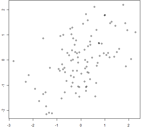
> plot(mvrnorm(100, c(0,0), matrix(c(1,mycor,mycor,1), 2), empirical=TRUE))

Figure 1: 100 random normals with sample correlation = 0.5
Figure 1 shows an example of the plot command in action.  (The figure cheats slightly by setting xlab and ylab to the empty string.)  You can recall the plot command and re-execute it several times to get a sense of how variable the same sample correlation can look.  You can then change the correlation or the sample size.

Now that we know what a variance matrix is, how do we go about getting one?  We have to estimate it. In the abstract statistical setting we estimate a variance matrix using a matrix of data.  The rows are observations, the columns are variables.  The result is a variance matrix that is number of variables by number of variables.  The assumption is that each observation is independent from the others, and they all have the same distribution.  In particular they all come from the same variance matrix.

We’ll start with a matrix of returns: times (trading days, for instance) in the rows, assets in the columns.  But here is where we and textbook statistics part ways.

The means of returns at different times are (presumably) not the same, like statisticians demand.  But they are close enough that this issue is not worth worrying about.

In market data there is the phenomenon of volatility clustering.  Volatility jumps up during crises and then gradually dies back down again.  The dying down is decidedly non-smooth.

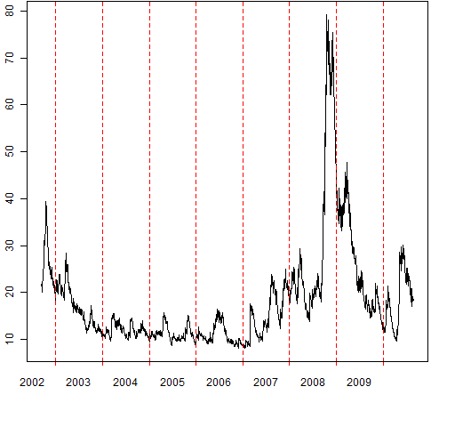
Figure 2: Approximate S&P 500 volatility for 2000 days up to 2010-Aug-23
Figure 2 provides a feel for volatility clustering.  The estimate of volatility was done with a rather crude model, but if we magically had a picture of the true volatility, the overall features would be very similar.

Correlations are dynamic as well.  In general they also increase during crises.

For these reasons using as long of a history as possible to estimate the variance matrix is not a good plan.  We only want to use current data.  What does “current” mean?  Excellent question.

The classical statistics set-up demands that we have more observations than variables (more time periods than assets in our case).  It isn’t that we can’t do the calculation if there are fewer times than assets, it’s that we might not like what we get.  The technical terms for what we get is a singular matrix — one that is not positive-definite.  The practical effect is that the variance matrix says that there exist portfolios with zero volatility. That’s a place not to go — there be dragons.

There are several ways to get around this problem.  We’ll save that discussion for another post or two.

One more caution that you’ll find in the statistics literature is that correlation is only about linear relationships.  There is the possibility of zero correlation, but a strong relationship.  Perhaps there are other opinions, but I don’t think we need to worry about this. Relationships are continuously in flux so we can only ever get an approximation anyway.  A linear approximation is about all we can hope for.

Let”s review:

• The true variance matrix is constantly changing.
• In many cases we will have fewer time periods than assets.

The first point suggests that what we want (most often) is a prediction for some future time period rather than an estimation of the past.  The second suggests that that prediction is going to be noisy.  Very noisy to a statistician’s eye.

Using a financial perspective, the prediction error of the variance matrix is rather modest though.  Predicting returns is close to impossible, so relatively speaking the variance matrix is predicted with brilliant accuracy.

Subscribe to the Portfolio Probe blog by Email