Should you use daily or monthly returns to estimate volatility?
Does garch explain why volatility estimated with daily data tends to be bigger than if it is estimated with monthly data?
Previously
There are a number of previous posts — with the variance compression tag — that discuss the phenomenon of volatility estimated with daily data tending to be higher than if estimated with monthly data. In particular, there is “The mystery of volatility estimates from daily versus monthly returns”. Quite apropos of the current post is “The volatility mystery continues”.
There is also “A practical introduction to garch modeling”.
Experiment
Here’s the idea: Simulate 3 years of daily data from a garch model (of the S&P 500). Then estimate the volatility over that three years using both the daily returns and the data aggregated into monthly returns. The key thing with a garch simulation is that we also have the true value of the volatility (unlike market volatility which we never get to see directly).
Three simulations of 1000 series each were performed. The difference between the simulations was the starting volatility:
- average volatility (and hence moderate)
- small (the 1% quantile of volatility of a long history)
- large (the 99% quantile)
Results
Precision
There is a striking difference between the accuracy of volatility estimated with daily data versus monthly data. Figures 1 and 2 show the actual volatility versus the estimates for the moderate volatility simulation.
Figure 1: Volatility estimates from daily data versus true volatility in the moderate volatility simulation. 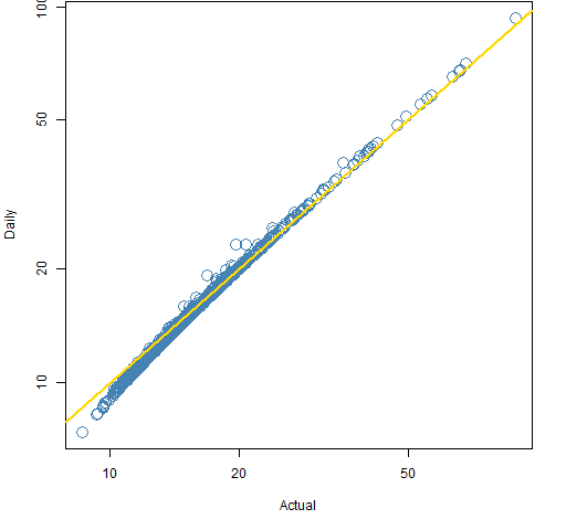
Figure 2: Volatility estimates from monthly data versus true volatility in the moderate volatility simulation. 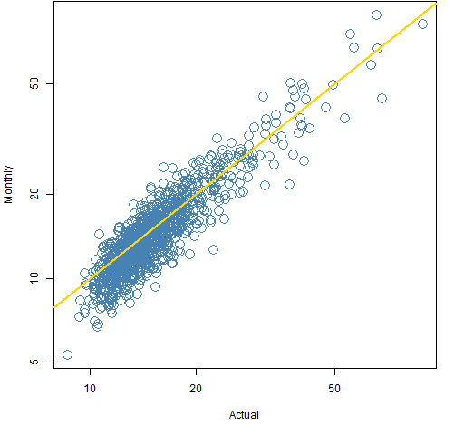 The plots for the small and large volatility simulations (Figures 3 through 6) tell the same story.
Figure 3: Volatility estimates from daily data versus true volatility in the small volatility simulation. 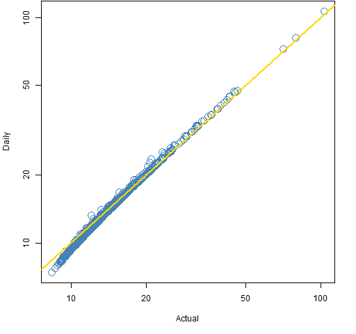
Figure 4: Volatility estimates from monthly data versus true volatility in the small volatility simulation. 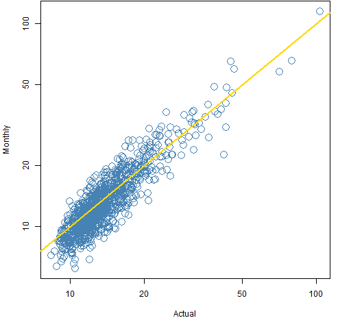
Figure 5: Volatility estimates from daily data versus true volatility in the large volatility simulation. 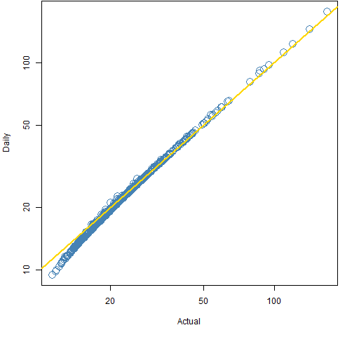
Figure 6: Volatility estimates from monthly data versus true volatility in the large volatility simulation. 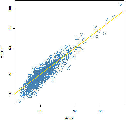
Bias
Figures 7 and 8 show the bootstrap distributions of the mean bias of the daily and monthly estimates in the three simulations. The bias is of volatility expressed in percent.
Figure 7: Bootstrap distributions of the mean of daily estimate minus actual volatility. 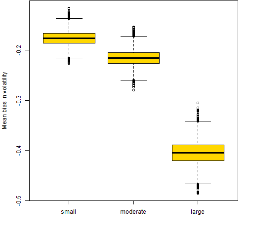
Figure 8: Bootstrap distributions of the mean of monthly estimate minus actual volatility. 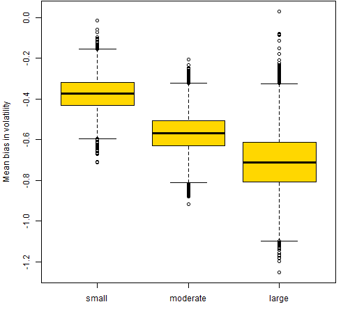
The bias in the monthly estimates is less than one percentage point, and the difference between daily estimates and monthly estimates is even less than that.
Limitations
The garch model does not exactly replicate how markets operate. But for these purposes it is probably pretty close.
Questions
Are there particular reasons to be suspicious of these results?
What is the explanation for the daily estimates to be biased downward for very small actual volatilities?
Summary
For a garch model the daily estimates of volatility are clearly more accurate than the monthly estimates. It seems hard to believe that the model is wrong enough to overthrow that in reality.
The garch simulations do exhibit a small amount of variance compression (monthly estimates are smaller than daily). However, it doesn’t look like there is as much in the garch model as in market data. I think there is something else happening in the market as well.
Appendix R
garch estimation
See the rugarch section of “A practical introduction to garch modeling” for how the garch model was estimated. It was a garch(1,1) with t-distributed errors.
It is like the one shown in Appendix R of “The volatility mystery continues”.
garch simulation
To simulate using the average volatility:
spxgsim0 <- ugarchsim(spxgar, n.sim=756, m.sim=1000,
   startMethod="unconditional")
To start with the most recent volatility, you would say:
startMethod="sample"
(which seems like a confusing name for the choice to me).
To start with the large volatility, do:
spxgsim01 <- ugarchsim(spxgar, n.sim=756, m.sim=1001,
   presigma=quantile(spxgarvol, .01)/100 / sqrt(252))
This command includes an attempt to save me from myself. Slightly different numbers (1000, 1001, 1002) are used in the three simulations. This can sometimes signal that something is wrong if objects are inappropriately mixed.
extract from simulation objects
The (non-transferable) trick of getting relevant data out of rugarch simulation objects is to use as.data.frame:
spxgsim0s <- as.data.frame(spxgsim0, which="series")
spxgsim0v <- as.data.frame(spxgsim0, which="sigma")
volatility estimation
The two objects created just above are the inputs to the function that gives us our comparison of volatilities:
pp.volcompare <- function(series, sigma, month=21)
{
  # compare volatility estimates
  # placed in public domain 2012 by Burns Statistics
  #
  # testing status:
  # slightly tested, in that monthly returns check
  # results seem to make sense

  series <- as.matrix(series)
  sigma <- as.matrix(sigma)
  stopifnot(all(dim(series) == dim(sigma)),
            nrow(series) %% month == 0)

  ans <- array(NA, c(ncol(series), 3), list(NULL,
            c("Daily", "Monthly", "Actual")))
  ans[, "Daily"] <- apply(series, 2, sd) * sqrt(252)
  ans[, "Actual"] <- sqrt(colSums(sigma^2) *
    252/nrow(sigma))
  nmon <- nrow(series) / month
  mseries <- crossprod(kronecker(diag(nmon),
    rep(1, month)), series)
  ans[, "Monthly"] <- apply(mseries, 2, sd) *
    sqrt(252/month)
  ans
}
The bit with kronecker is some matrix magic that gets us the monthly returns that we want. One hint about how this works is that
diag(36)
is the R way of getting the 36 by 36 identity matrix.
Another way of collapsing to monthly returns that is more flexible is:
crossprod(diag(36)[rep(1:36, each=21),], series)
We can generalize this formulation to months that have different numbers of days.
use the compare function
The function is actually used like:
spxgsim0comp <- pp.volcompare(spxgsim0s, spxgsim0v)
The results look like:
> head(spxgsim0comp)
          Daily   Monthly    Actual
[1,] 0.09791878 0.1441274 0.1057857
[2,] 0.21882895 0.2677690 0.2176373
[3,] 0.14704830 0.1454526 0.1499731
[4,] 0.15218896 0.1361271 0.1541258
[5,] 0.14157192 0.1166982 0.1454488
[6,] 0.15529995 0.2052485 0.1573691
bootstrap mean bias
The bootstrapping does a little preparatory work:
diff0da <- (spxgsim0comp[, "Daily"] -
  spxgsim0comp[, "Actual"]) * 100
diff0ma <- (spxgsim0comp[, "Monthly"] -
  spxgsim0comp[, "Actual"]) * 100
The bootstrapping proper is:
boot0da <- numeric(1e4)
for(i in 1:1e4) {
  boot0da[i] <- mean(sample(diff0da, 1000, replace=TRUE))
}
boot0ma <- numeric(1e4)
for(i in 1:1e4) {
  boot0ma[i] <- mean(sample(diff0ma, 1000, replace=TRUE))
}
The boxplots are created like:
boxplot(list(small=boot01da, moderate=boot0da,
   large=boot99da), col="gold",
   ylab="Mean bias in volatility")
Hi,
First, thank you for your interesting posts that I regularly come across at R-Bloggers!
I was wondering if in the above simulation-reestimation procedure the more erratic behavior of monthly estimates is just due to less data and hence higher standard errors in the estimates?
Thomas,
Thanks for your interest.
My answer to your question is: yes and no.
In a sense there is the same amount of data in the daily and monthly datasets. The difference is that the aggregation to monthly hides information. That won’t matter for the expected return, but it does matter for volatility. We have 756 observations with daily data but only 36 observations with monthly data to see the variability.
The folklore in finance is that aggregating to lower frequency is better because the higher frequency data is “noisy”. However, the noisiness is precisely what we want to know about when estimating volatility.
The folklore has a point if there is autocorrelation between observations. That is true of intraday data — there is significant seasonality (in terms of volatility) within days. But daily data is very close to having no autocorrelation.
Hi,
thanks for some interesting thoughts and points regarding data frequency for volatility estiamtion.
My question is: how would you use daily return data to make monthly volatility estimates with a GARCH(1,1) model? It seems like a waste of information to only base it on the monthly return and I’m not sure about producing a daily forecast for each day of the month and then sum them up. I hope you have understood my question=)
Regards Richard
I have no evidence on what are the better procedures. It’s an interesting question.
Dear Pat,
I have tried to replicate your results, but I cannot run this function: spxgsim01 <- ugarchsim(spxgar, n.sim=756, m.sim=1001,
presigma=quantile(spxgarvol, .01)/100 / sqrt(252)).
I do not have "spxgarvol". Can you please share the codes before you do the ugarchsim? I assume that you have used spec and ugarchfit prior to using ugarchsim
Interestingly and unfortunately I don’t have ‘spxgarvol’ either. I don’t know what happened there.