Value at Risk and Expected Shortfall are common risk measures.  Here is a quick explanation.

Ingredients

The first two ingredients are each a number:

1. The time horizon — how many days do we look ahead?
2. The probability level — how far in the tail are we looking?

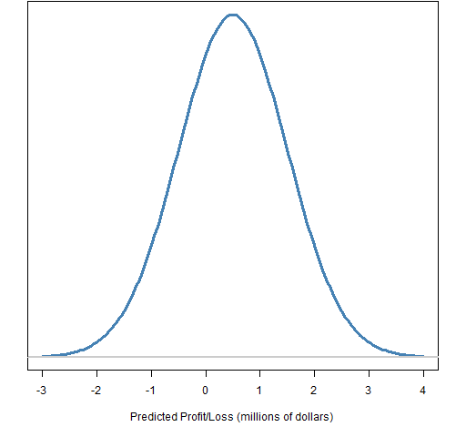
Ingredient number 3 is a prediction distribution of profit and loss given the time horizon, an example is shown in Figure 1.

Figure 1: A predicted profit and loss distribution.

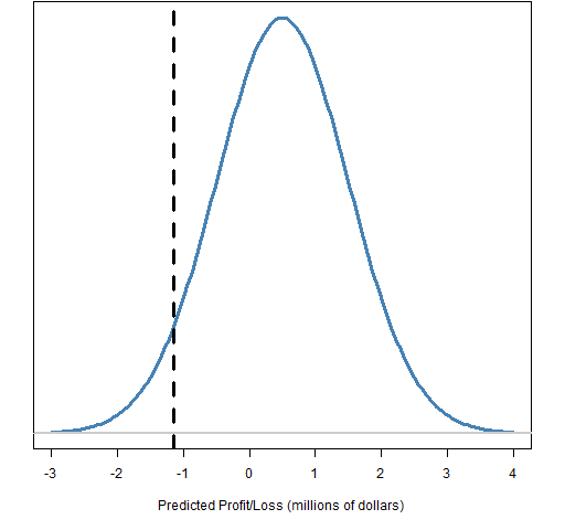
The fourth ingredient is the quantile of the prediction given the probability level.

Figure 2: Predicted profit and loss distribution with the quantile marked.

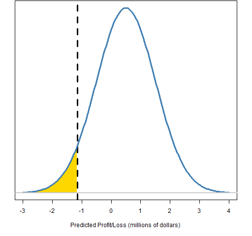
The final ingredient (not used by Value at Risk) is the tail beyond the quantile.

Figure 3: Predicted profit and loss distribution with the quantile and tail marked.

The measures

The result is a single number, which is some amount of money.

Value at Risk (VaR) is the negative of the predicted distribution quantile at the selected probability level.  So the VaR in Figures 2 and 3 is about 1.1 million dollars.

Expected Shortfall (ES) is the negative of the expected value of the tail beyond the VaR (gold area in Figure 3).  Hence it is always a larger number than the corresponding VaR.

Aliases

As far as I know, Value at Risk is always Value at Risk.

Expected Shortfall

Expected Shortfall has a number of aliases:

• Conditional Value at Risk (CVaR)
• Mean Shortfall
• Mean Excess Loss

I find “Conditional Value at Risk” to be confusing.  I can see people thinking it is a Value at Risk given some condition rather than the expected loss beyond the Value at Risk.

Mean Excess Loss seems the most descriptive name.

Above we see one concept with several names.  Below we see one name with multiple concepts.

Expected Shortfall has other meanings.  Rather than expectation beyond VaR, it can be expectation beyond some requirement (which fits the name better than the concept we are describing).

Probability level

Some people say 95% when I say 5%.  No worries.  We are always dealing with the tail — meaning something definitely less (in my terminology) than 50%.  If a level is at the wrong end for your taste, just think one minus it.

Abbreviations

The abbreviation for Value at Risk has the potential for confusion with two other concepts:

• variance
• vector autoregression

All of these can be kept from colliding with a convention on capitalization:

• VaR: Value at Risk
• var: variance
• VAR: vector autoregression

Road to estimation

initial ingredients

There are two initial ingredients:

• the asset positions in the portfolio
• the price history of the assets involved

derived ingredients

The portfolio positions plus the current prices yields the portfolio weights.

The price history matrix is used to get the return history matrix.

estimation and collapse

We are starting with information at the asset level and we need to end up with a one-dimensional view at the portfolio level.

Perhaps there are hybrid solutions, but essentially either we need to estimate and then collapse to one dimension, or we need to collapse to one dimension and then estimate.

estimate then collapse

In this setting we need to estimate a variance matrix.  This will often be a factor model, but could be some other estimate.

The portfolio variance is computed using the variance matrix and the portfolio weights.

The primary reason to go this route is to break the VaR or ES into pieces based on the factors.

An alternative to estimating a static model is to fit a multivariate garch model.  The VaR or ES could then be found using either a prediction of the garch model or a simulation of it.  This is unlikely to be a viable choice.

collapse then estimate

Here we use the current weights to create a history of portfolio returns.

There are a number of ways to get the prediction distribution given the portfolio return history:

• fit an assumed distribution
• simulation (use the empirical distribution over some time period)
• garch prediction
• garch simulation

If you assume a normal distribution, then you can estimate the standard deviation to get your prediction distribution.  If you assume a t-distribution, then you need additionally to estimate the degrees of freedom or assume the degrees of freedom.

What is often called the simulation method is really just using the empirical distribution of some specific number of portfolio returns.

Using a univariate garch model can be quite a good way to estimate VaR and ES.

Alternatively for VaR, there is a clever approach which is to directly estimate the quantile without worrying about the distribution.  This is CaViaR by Engle and Manganelli.

Summary

This introduction to Value at Risk and Expected Shortfall is just the beginning of the topic.

They are very simple concepts — that is why they are popular.  They are probably too simple.

Appendix R

The R language is quite a suitable environment for VaR and ES.

filled areas

You may be wondering how to fill an area in a plot as is done in Figure 3.  The trick is to use the polygon function.  Here is the function that created Figure 3:

function (filename = "preddisttail.png") 
{
    if(length(filename)) {
        png(file=filename, width=512)
        par(mar=c(5,2, 0, 2) + .1)
    }
    xseq <- seq(-3, 4, length=200)
    pd <- dnorm(xseq, mean=.5, sd=1)
    plot(xseq, pd, type="l", col="steelblue", lwd=3, 
        yaxt="n", ylab="", 
        xlab="Predicted Profit/Loss (millions of dollars)")
    abline(v=qnorm(.05, mean=.5, sd=1), lty=2, lwd=3)
    xseqt <- xseq[xseq < qnorm(.05, mean=.5, sd=1)]
    polygon(c(xseqt, max(xseqt)), c(dnorm(xseqt, 
        mean=.5, sd=1), 0), col="gold", border=NA)
    lines(xseq, pd, type="l", col="steelblue", lwd=3)
    abline(h=0, col="gray80", lwd=2)

    if(length(filename)) {
        dev.off()
    }
}

portfolio variance calculation

The R command to get the portfolio variance given the variance matrix and the weight vector is:

weight %*% varianceMatrix %*% weight

This assumes that the weight vector is perfectly aligned to the variance matrix.  A safer command would be:

weight %*% varianceMatrix[names(weight), 
   names(weight)] %*% weight