Overfitting is a problem when trying to predict financial returns. Perhaps you’ve heard that before. Some simple examples should clarify what overfitting is — and may surprise you.
Polynomials
Let’s suppose that the true expected return over a period of time is described by a polynomial.
We can easily do this in R. The first step is to create a poly object:
> p2 <- poly(1:100, degree=2)
> p4 <- poly(1:100, degree=4)
(Explanations of R things are below in Appendix R.)
Now we can create our true expected returns over time:
> true2 <- p2 %*% c(1,2)
> true4 <- p4 %*% c(1,2,-6,9)
> plot(1:100, true2)
> plot(1:100, true4)
Figure 1: Plot of the quadratic polynomial.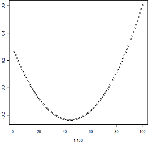
Figure 2: Plot of the fourth degree polynomial.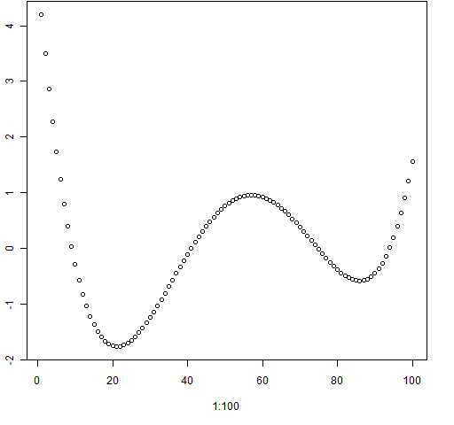
Polynomial regression, no noise
We can do regressions with linear and quadratic models on the quadratic data:
> reg.t2.1 <- lm(true2 ~ I(1:100))
> reg.t2.2 <- lm(true2 ~ p2)
> plot(1:100, true2)
> abline(reg.t2.1, col="green", lwd=3)
> lines(1:100, fitted(reg.t2.2), col="blue", lwd=3)
Figure 3: Quadratic data with regressions on full data.
But this isn’t really the problem we are faced with when predicting returns. In practice we have a history of returns and we want to predict future returns. So let’s use the first 70 points as the history and the final 30 as what we are predicting. And let’s use the degree 4 data this time:
> days <- 1:70
> reg.pt4.1 <- lm(true4[1:70] ~ days)
> reg.pt4.2 <- lm(true4[1:70] ~ poly(days, 2))
> reg.pt4.4 <- lm(true4[1:70] ~ poly(days, 4))
We can then see how well these predict the out of sample data.
Figure 4: Fits and predictions for the degree 4 data.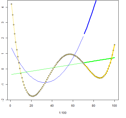
Figure 4 might hold your first surprise. The linear model is conceptually farther from a fourth degree polynomial than the quadratic model, but the linear model clearly predicts better than the quadratic. The quadratic prediction for time 100 is seriously too high — way off scale.
Polynomial regression, noise added
Returns, of course, come with noise. So lets add some noise and see how the predictions do.
> noise4 <- true4 + rnorm(100, sd=.5)
Figure 5 shows what this new data looks like. The shape of the fourth degree polynomial is still quite visible. It is nowhere near as noisy as real returns.
Figure 5: The fourth degree data with noise added.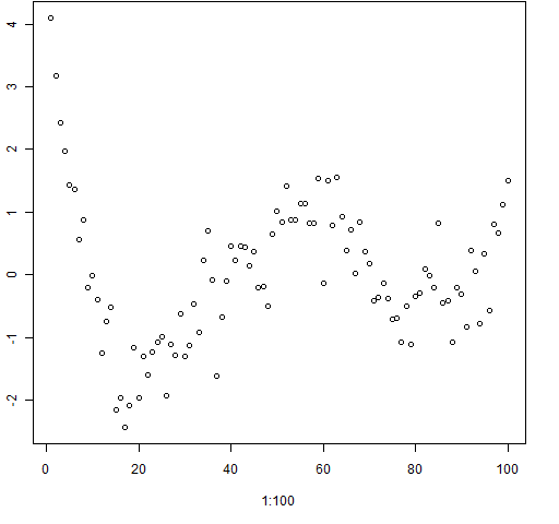
So what are the predictions like? Figure 6 shows us.
Figure 6: The noisy fourth degree data with fits and predictions. The dotted black line is the actual expected value.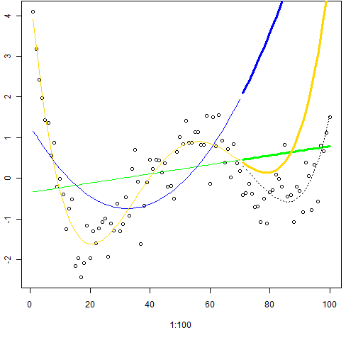
This time the linear prediction not only beats the quadratic model but it beats the “right” model as well. The fourth degree prediction starts off a little better but then goes off the rails.
Polynomial regression, all noise
Let’s try our exercise on pure noise:
> noise0 <- rnorm(100)
> reg.n0.1 <- lm(noise0[1:70] ~ days)
> reg.n0.2 <- lm(noise0[1:70] ~ poly(days, 2))
> reg.n0.4 <- lm(noise0[1:70] ~ poly(days, 4))
This is much more similar to returns, except returns do not have a normal distribution.
Figure 7: The all-noise data with fits and predictions.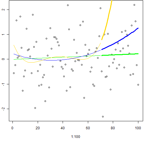 The polynomial fits have predictions that go weird.
Moral of the story
The more parameters in your model, the more freedom it has to conform to the noise that happens to be in the data. Even knowing the exact form of the generating mechanism is no guarantee that the “right” model is better than a simpler model.
To some extent the examples presented here are cheating — polynomial regression is known to be highly non-robust. Much better in practice is to use splines rather than polynomials. But that doesn’t take away from the fact that an over-sharpened knife dulls fast.
Epilogue
Appendix R
Polynomials
The p2 object is a matrix with 100 rows and two columns while p4 is a matrix with 100 rows and four columns. Conceptually p2 is the same as the matrix that has 1 through 100 in the first column and the square of those numbers in the second column. In R that would be:
> cbind(1:100, (1:100)^2)
There are two main differences between p2 and the matrix above:
- the columns are scaled by poly
- the columns are made orthogonal by poly
It’s the second property that is the more important. It reduces numerical problems, and it aids in the interpretation of results. We can see that the columns are orthogonal by looking at the correlation matrix:
> cor(p4)
1 2 3 4
1 1.000000e+00 -2.487566e-17 2.175519e-17 -1.455880e-17
2 -2.487566e-17 1.000000e+00 1.026604e-18 -3.303428e-18
3 2.175519e-17 1.026604e-18 1.000000e+00 -5.773377e-18
4 -1.455880e-17 -3.303428e-18 -5.773377e-18 1.000000e+00
We can see it better by using a little trick to get rid of the numerical error:
> zapsmall(cor(p4))
1 2 3 4
1 1 0 0 0
2 0 1 0 0
3 0 0 1 0
4 0 0 0 1
Polynomial regression
You’ll notice that we changed the formulas when we switched from fitting all of the data to fitting only part of the data and predicting. The predict function really really wants its newdata argument to be a data frame that has variables that are in the formula.
The code that created Figure 7 is:
plot(1:100, noise0)
lines(1:70, fitted(reg.n0.1), col="green")
lines(1:70, fitted(reg.n0.2), col="blue")
lines(1:70, fitted(reg.n0.4), col="gold")
lines(71:100, predict(reg.n0.1,
newdata=data.frame(days=71:100)), col="green", lwd=3)
lines(71:100, predict(reg.n0.2,
newdata=data.frame(days=71:100)), col="blue", lwd=3)
lines(71:100, predict(reg.n0.4,
newdata=data.frame(days=71:100)), col="gold", lwd=3)
Pingback: Monday links: reputation and returns Abnormal Returns
Pingback: Highlights of R in Finance 2012 | Portfolio Probe | Generate random portfolios. Fund management software by Burns Statistics
Pingback: A practical introduction to garch modeling | Portfolio Probe | Generate random portfolios. Fund management software by Burns Statistics
Usually, students can just use either smartphones or level-and-shoot” cameras and it
may not be essential for them to make use of skilled gear.
This time the driver stopped the automotive
at street side and advised us our agreed the taxi fare
was EUR 35 per particular person instead. And my husband
returned him the EUR 15 he gave at first, we modified another taxi.
As your premium outlet for hookahs and hookah accessories, we’re proud to supply prime-of-the-line hookahs, water pipes,
and flavored tobacco for hookah enthusiasts of all types.
We’ve a method of hookah for everyone, from first-timers
to skilled hookah aficionados.
A workforce of Kansas State College students partnered with the Union Program Council and the Workplace of the
President to carry the TEDx occasion to Manhattan.
Pingback: rcs在lm()模型中生成错误的预测 - 实战宝典