Additional views of the stability of skewness and kurtosis of equity portfolios.
Previously
A post called “Four moments of portfolios” introduced the idea of looking at the stability of the mean, variance, skewness and kurtosis of portfolios through time.
That post gave birth to a presentation at the London Quant Group.
That talk gave birth to several questions — the present post explores one of them.
Pictures
A critique of the plots like Figures 3 and 4 of “Four moments of portfolios” was that there is autocorrelation in the ranks from one day to the next because they are based on 250-day windows. Figures 1 through 4 here change that — these look at the mean absolute difference of days that are 250 days apart. So the two ranks in the difference are formed in blocks that are adjacent but not overlapping.
Figure 1: Mean absolute value of the differences of ranks 250 days apart for the 200-name random portfolios. 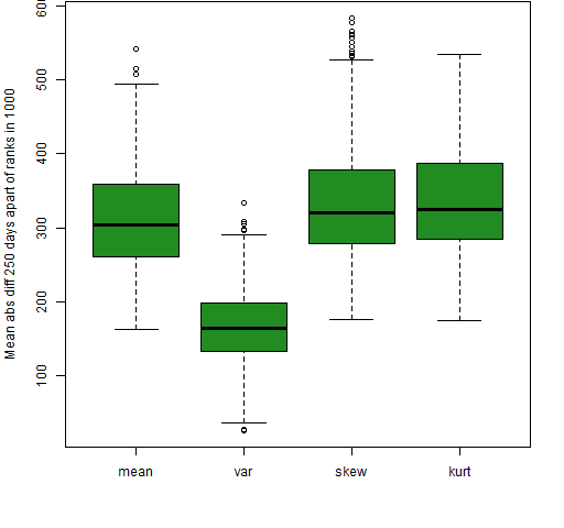
Figure 1 is the same as Figure 4 of “Four moments of portfolios” except for the lag in the difference. When there are overlapping windows, the higher moments look more stable than the mean (but see below); while in the non-overlapping case here, they have ever so slightly worse stability than the mean.
Figure 2: Mean absolute value of the differences of ranks 250 days apart for the 200-name random portfolios using returns Winsorized at 3 (robust) standard deviations. 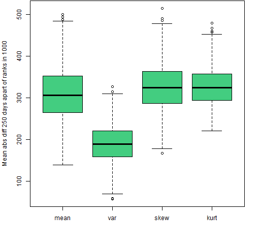
Comparing Figure 2 with Figure 1 we see Winsorization to have a minimal effect for the higher moments when the windows are not overlapping. In the overlapping case Winsorization made the higher moments look much less stable.
Figure 3: Mean absolute value of the differences of ranks 250 days apart for the 200-name random portfolios using returns with and without Winsorizing at 3 (robust) standard deviations for the mean and variance. 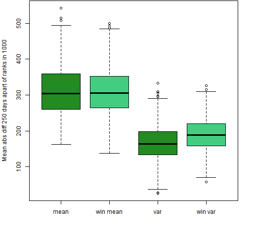
In Figure 3 we see that Winsorization still makes the variance less stable for non-overlapping windows, but the difference is more muted. Figure 4 shows that for skewness and kurtosis in the non-overlapping case the only effect of Winsorization seems to be to decrease variability slightly.
Figure 4: Mean absolute value of the differences of ranks 250 days apart for the 200-name random portfolios using returns with and without Winsorizing at 3 (robust) standard deviations for skewness and kurtosis. 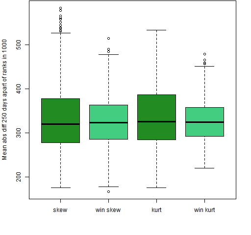
Autocorrelation
One of the questions during the presentation was why are the outliers for the mean all on the upside and all the outliers for the variance on the downside. It looks like Antonia Lim’s intuition of autocorrelation causing it seems believable — there is no such pattern in Figure 3 here. However, I still don’t understand the idea.
Total instability
We can see what to expect if there is no stability at all by randomly permuting the returns each day among the portfolios.
Figure 5: Mean absolute value of the differences of ranks on adjacent days for permuted returns. 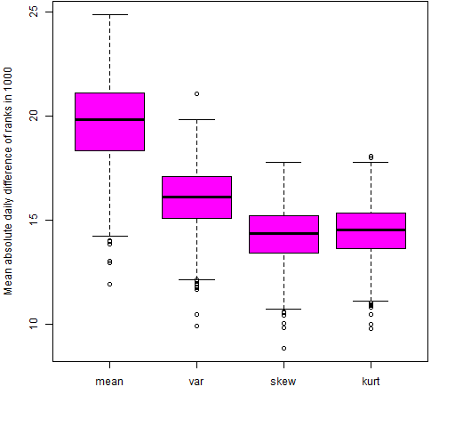
Figure 5 confirms Robert Macrae’s suggestion that the line of usefulness is downward sloping.
Figure 6: Mean absolute value of the differences of ranks 250 days apart for permuted returns. 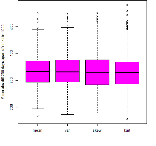
Comparing Figures 3 and 4 with Figure 6 suggests that the mean, skewness and kurtosis might have a sliver of stability.
Questions
Why is Antonia right about autocorrelation?
Why is Robert right about differing baselines in the overlapping window case (Figure 5)?
Summary
This new view makes skewness and kurtosis appear even less useful in equities than before. Any stability they have on this time scale is minimal. However, there might be more stability on a shorter time scale.
Epilogue
and they like some wild river flow as we go further in
from “Further In” by Greg Brown
Appendix R
Computations and plots were done in R.
lagged differences
It was trivial to change from doing a difference between adjacent days and a difference between days 250 apart:
mrngmean250d250.w200.lo <- apply(rankmean250.w200.lo, 2,
   function(x) mean(abs(diff(x, lag=250))))
Usually diff is only used with its first argument but there are two more arguments that are sometimes of interest. In this case the lag argument was what was needed.
> diff(1:9)
[1] 1 1 1 1 1 1 1 1
> diff(1:9, lag=3)
[1] 3 3 3 3 3 3
permute returns
The rows of the original return matrix were permuted (independently of each other) with:
permrret.w200.lo <- t(apply(rret.w200.lo, 1, sample))
The sample function with only one argument does a random permutation. The transpose of the result of this apply call is necessary for a reason explained in Circle 8.1.47 of The R Inferno.
