What good are the skewness and kurtosis of portfolios?

Previously

The post “Cross-sectional skewness and kurtosis: stocks and portfolios” looked at skewness and kurtosis in portfolios.  The key difference between that post and this one is what distribution is being looked at.

The previous post specified a single time and looked at the distribution across portfolios.  This post specifies a particular portfolio and looks at the distribution across a number of days.

Set up

Daily adjusted prices on 443 large cap US stocks from the beginning of 2004 to the end of 2012 are used.  Two sets of random portfolios are produced, each containing 1000 portfolios.  The portfolios are created as of the start of 2004.

The first set has constraints:

• exactly 20 names
• no asset has a weight at inception greater than 10%
• no asset in the portfolio has weight at inception less than 1%

The second set has constraints:

• exactly 200 names
• no asset has a weight at inception greater than 3%
• no asset in the portfolio has weight at inception less than 0.1%

The mean, variance, skewness and kurtosis of the log returns is found for each portfolio over rolling windows of 250 days. On each day for each moment the rank across the portfolios in the set is found.

For example, consider the kurtosis of the 20-name portfolios on the last trading day of 2005.  The kurtosis for each portfolio is based on almost all its daily returns for the year 2005.  The portfolio with the smallest kurtosis on this day is given rank 1, the portfolio with the second smallest kurtosis on this day gets rank 2, and so on.  The portfolio with the largest kurtosis on the day gets rank 1000.

Moment stability

One question of interest is how persistent are the rankings of the moments.  If a portfolio has recently had relatively small kurtosis among its peers, can we depend on it to continue to have relatively small kurtosis?

Figures 1 and 2 provide an answer by looking at the range of ranks that each portfolio takes on over the 9 years.  If a portfolio has the smallest value at one time and the largest value at another time, then it will have a rank range of 999.  Each boxplot displays values for 1000 portfolios.

Figure 1: Range of ranks out of 1000 for the 20-name random portfolios. 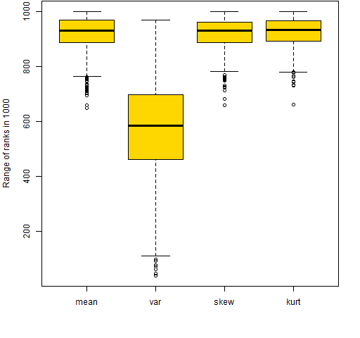 Figure 2: Range of ranks out of 1000 for the 200-name random portfolios.  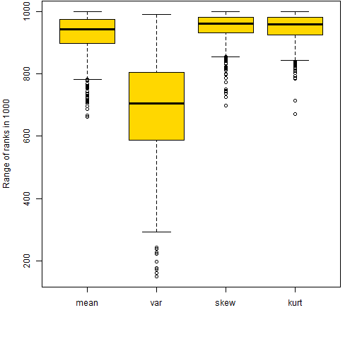Figures 1 and 2 are very similar.  They show that skewness and kurtosis look very much like the mean in this regard — all three of these moments move around substantially over the 9 years.  In contrast the variance is much more stable.

The range of the ranks is a rather crude measure.  We would get the same range if a portfolio went smoothly from largest to smallest over the nine years as if it switched between largest and smallest every day.

A less crude measure is the mean change in rank each day over the nine years — that is shown in Figures 3 and 4.

Figure 3: Mean absolute value of the daily differences of ranks out of 1000 for the 20-name random portfolios. 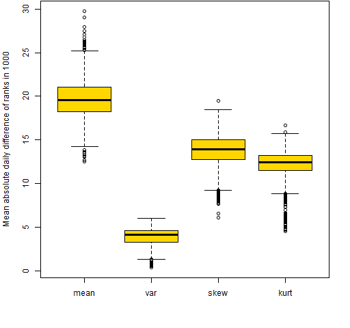 Figure 4: Mean absolute value of the daily differences of ranks out of 1000 for the 200-name random portfolios.  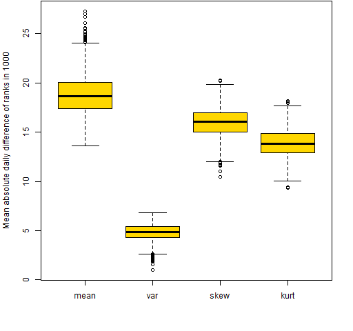By this new measure skewness and kurtosis are not as variable as the mean return, but they are still very much more variable than the variance.

Variance stability

I hypothesized that low variance would be more persistent than high variance.  Figures 5 and 6 seem to say that my hypothesis is wrong.

Figure 5: Mean absolute value of the daily differences of ranks of the variance out of 1000 for the 20-name random portfolios versus mean rank of the variance. 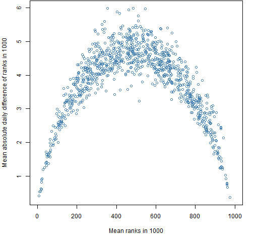 Figure 6: Mean absolute value of the daily differences of ranks of the variance out of 1000 for the 200-name random portfolios versus mean rank of the variance.  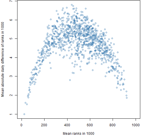Figure 7 shows variances of  the 20-asset portfolios from one year to the next.  This is a case where the correlation is a poor description.  In general variances are lower in 2012 than in 2011, but there is a sub-population where the variances are higher.  The sub-population distorts the value of the correlation.  Or more accurately: the correlation hides the complexity of the relationship.

Figure 7: 2012 variances versus 2011 variances for the 20-name portfolios.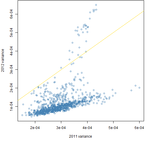 

Summary

We’ve seen that there is little predictability of skewness and kurtosis for the portfolios relative to similar portfolios.  This is in the realm of large cap US equities.  I suspect this is probably true of just about any equity universe and set of constraints (but I’ve been wrong before).  Some other assets may well have reasonable predictability.

The results seem quite significant to me for the prospects of doing portfolio optimization with higher moments.  Ranking among portfolios is precisely what optimization wants to do.

Skewness and kurtosis will not be useful for problems — as here — where they fail to be persistent in terms of rank among portfolios. That is not to say that there can’t be ways to predict skewness and kurtosis to a useful degree, but using historical returns seems an unlikely route for at least some assets.  We’ll have to turn back or build a new plan.

Epilogue

This minute would crack
And I could go through
And walk out in time
Where no one has been

from “It Isn’t Gonna Be That Way” by Steve Forbert

Updates

2013 December: Further adventures with higher moments

Appendix R

The computations and graphics were done in R.

generate random portfolios

The first two steps — generating random portfolios and computing the returns of the portfolios — requires the Portfolio Probe software, hence:

require(PortfolioProbe)

The generation of the portfolios is done via:

rp.w020.lo <- random.portfolio(number.rand = 1000, 
   prices = initclose[1,], gross=1e7,
   long.only=TRUE, port.size=c(20,20),
   max.weight=.1, min.weight.thresh=.01)

rp.w200.lo <- random.portfolio(number.rand = 1000, 
   prices = initclose[1,], gross=1e7,
   long.only=TRUE, port.size=c(200,200),
   max.weight=.03, min.weight.thresh=.001)

compute returns

The initclose object is a matrix of closing prices over the 9 years (assets in columns, days in rows).  This matrix is used to compute the portfolio returns:

rret.w020.lo <- valuation(rp.w020.lo, 
   prices=initclose, returns="log")
rret.w200.lo <- valuation(rp.w200.lo, 
   prices=initclose, returns="log")

compute skewness and kurtosis

Now the skewness and kurtosis for rolling 250-day windows is computed for the portfolios.  This depends on a package:

require(moments)

First, objects are created to hold the results and then they are populated with values:

skew250.w020.lo <- rret.w020.lo
skew250.w020.lo[] <- NA
kurt250.w200.lo <- skew250.w200.lo <- 
   kurt250.w020.lo <- skew250.w020.lo

tseq <- -249:0
for(i in 250:nrow(rret.w020.lo)) {
   tret <- rret.w020.lo[tseq + i,]
   skew250.w020.lo[i,] <- skewness(tret)
   kurt250.w020.lo[i,] <- kurtosis(tret)
   tret <- rret.w200.lo[tseq + i,]
   skew250.w200.lo[i,] <- skewness(tret)
   kurt250.w200.lo[i,] <- kurtosis(tret)
}

Finally the initial rows that are not used are removed.

skew250.w020.lo <- skew250.w020.lo[-1:-249,]
kurt250.w020.lo <- kurt250.w020.lo[-1:-249,]
skew250.w200.lo <- skew250.w200.lo[-1:-249,]
kurt250.w200.lo <- kurt250.w200.lo[-1:-249,]

An alternative would have been to create the objects to be their final size, but the current method is less prone to error.

compute mean and variance

An excuse to show the mean and variance computed separately from skewness and kurtosis could be that the computation has a subtle difference.  The real reason is that I started out thinking only about skewness and kurtosis and realized when I got some results that mean and variance should be in the mix as well.

for(i in 250:nrow(rret.w020.lo)) {
   tret <- rret.w020.lo[tseq + i,]
   mean250.w020.lo[i,] <- apply(tret, 2, mean)
   var250.w020.lo[i,] <- apply(tret, 2, var)
   tret <- rret.w200.lo[tseq + i,]
   mean250.w200.lo[i,] <- apply(tret, 2, mean)
   var250.w200.lo[i,] <- apply(tret, 2, var)
}

The difference in computation is that apply is used because mean and var do not operate on the columns of a matrix like skewness and kurtosis do.  Not shown is the code to create the mean and variance objects, nor trimming them afterwards.

compute ranks

An example of computing the ranks is:

rankskew250.w020.lo <- t(apply(skew250.w020.lo, 
   1, rank))

The result of apply needs to be transposed to get the same orientation because of a rather technical reason.  This is explained in Circle 8.1.47 of The R Inferno.

rank range

The range of ranks for each portfolio is computed like:

rrngmean250.w020.lo <- apply(rankmean250.w020.lo, 
   2, function(x) diff(range(x)))

mean absolute diff of rank

Similarly, the mean absolute value of the daily differences of ranks is found via:

mrngmean250.w020.lo <- apply(rankmean250.w020.lo, 
   2, function(x) mean(abs(diff(x))))

boxplots

The boxplots are produced with commands like:

boxplot(list(mean=rrngmean250.w020.lo, 
   var=rrngvar250.w020.lo,
   skew=rrngskew250.w020.lo,
   kurt=rrngkurt250.w020.lo),
   col="gold", ylab="Range of ranks in 1000")

yearly plots

The relationship from one year to the next for each of the years in the data can be explored with a command like:

for(i in 1:8) {
   plot(var250.w020.lo[1+ (i-1)*252,], 
      var250.w020.lo[1+ i*252,])
   abline(0,1, col="gold")
}

The last plot from this loop is essentially Figure 7.