Under the covers of strange bedfellows.

Previously

The idea of implied alpha was introduced in “Implied alpha — almost wordless”.

In a comment to that post Jeff noticed that the optimal portfolio given for the example is ever so close to the minimum variance portfolio.  That is because there is a problem with the example (though it sort of doesn’t matter).

It uses a risk aversion of 2.5 (which would be a risk aversion of 5 in some people’s minds).  That is a moderate risk aversion.  Except that the variance and the expected returns are scaled to percent.  This means that the risk aversion should have been divided by 100, but it wasn’t.  I should have given a risk aversion of 0.025.

Connection

This made me wonder about how implied alpha and minimum variance are connected.

Implied alpha tells you what you must have been thinking about the returns of the assets when you formed the portfolio (where “must” is subject to a list of assumptions and caveats).

A reason to do minimum variance is because you don’t think you know about returns.  Yet implied alpha goes against your wishes and tells you that you do have a view on returns — whether you like it or not.

What do the implied alphas of a minimum variance portfolio look like?

Computation

If w is the vector of weights for the portfolio and V is the variance matrix, then the implied alphas are:

cVw

for whatever positive value of c you like.

The assumption is that you are maximizing mean-variance utility, which is:

α’w – cw‘Vw

where c is the risk aversion (but some people have a division by 2).

In calculus you can find a maximum by taking the derivative of a function and setting it to zero.  If w were a scalar rather than a vector, we would have:

aw – cVw²

Taking the derivative with respect to w and setting it to zero gives us:

a – 2cVw = 0

It turns out that the analogous calculation works for vectors.  (That there is a 2 in this formula is sort of why some people divide by 2 in the utility formula.)

Sensibility

How can we make sense of Vw?

First, note that if all the correlations are positive (not so far-fetched) and the portfolio is long-only, then all numbers are positive and hence all the implied alphas will be positive.

Consider the implied alpha for the first asset.  It is the weight of the first asset times the variance of the first asset plus the sum of the covariances of the first asset with all the other assets times the respective weights.

Implied alphas that are relatively big are those that have large weights on large variances and covariances.  That is, they are the riskiest positions.  If a position is risky, we must think that it has good return potential or we’d scale it back.

Minimum variance

The following computations use 250 daily returns ending on 2013 May 17 on 441 large cap US equities to estimate the variance.

Let’s examine how much a change of variance estimate makes.  We’ll use a statistical factor model and Ledoit-Wolf shrinkage as competing estimates of the variance matrix.

We get the minimum variance portfolio (where the only constraint is that the portfolio is long-only) for each variance matrix.  The factor model optimization selected 36 assets to have positive weight while the Ledoit-Wolf optimization has 27 assets.  There are 24 assets in common, and the turnover (buys plus sells) to get from one to the other is 50%.

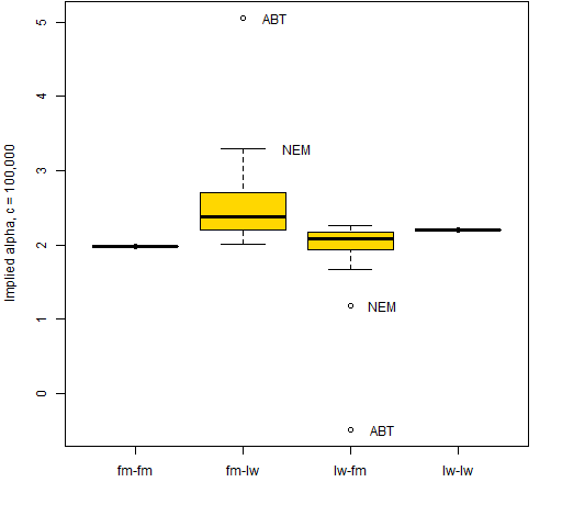
We then compute the implied alpha for each of these portfolios with each variance matrix.  Boxplots of these implied alphas are in Figure 1.

Figure 1: Boxplots of implied alpha vectors when optimizing and calculating implied alpha using a factor model (fm) or Ledoit-Wolf shrinkage (lw). The implied alphas computed with the same variance as was used in the optimization are all essentially equal.  That makes some sense — one way of getting the minimum variance portfolio is to do a mean-variance optimization where all the expected returns are equal.  In Portfolio Probe terminology the risk fractions are all equal.

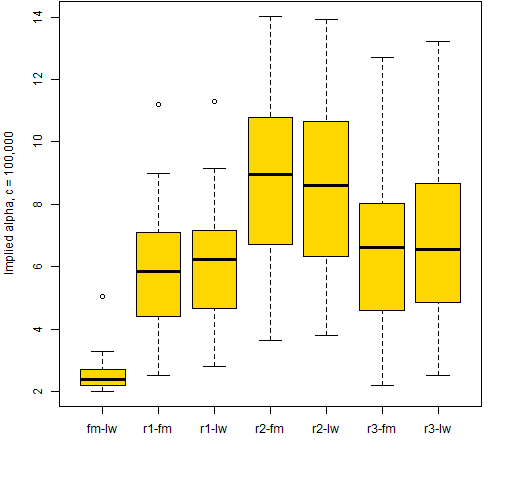
When we mix the variance matrices, then the implied alphas spread out.  But it isn’t clear how significant the spread is.  To get a sense of that, three weight vectors were randomly generated.  For each vector 30 random uniforms were generated, scaled to sum to 1, and then random assets from the universe were assigned.

Figure 2: Boxplots of implied alpha from factor model optimization and Ledoit-Wolf calculation (fm-lw) plus implied alphas from three random weight vectors. The answer seems to be that the spreads in Figure 1 are not entirely trivial.

But wait, there’s more.

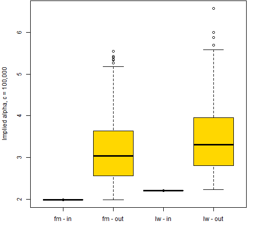
Figure 1 only looks at the implied alphas for the assets that have positive weights.  We can also get implied alphas for assets that are not in the portfolio.  Figure 3 shows implied alphas (using the same variance as in the optimization) for assets that are in the portfolio (positive weight) and out of the portfolio (zero weight).

Figure 3: Implied alphas for minimum variance portfolios divided by assets in the portfolio and those out of the portfolio. It appears that the “rule” is that the implied alphas for the assets in the minimum variance portfolio are all equal and the implied alphas for assets outside the portfolio are all larger.  This makes sense in that assets that are risky (have high implied alpha) are excluded.  However, it seems to foil the idea that doing a mean-variance optimization with the implied alphas would lead us back to the portfolio.

Question

How does the minimum variance portfolio “know” how many of the assets should be included?

Summary

Minimum variance portfolios have a strange but quite interesting set of implied alphas.

Epilogue

Did you ever have to finally decide?
And say yes to one and let the other one ride

from “Did you ever have to make up your mind?” by John Sebastian

Appendix R

Computations were in R.

create variance estimates

The variance estimates use functions in the BurStFin package:

require(BurStFin)
fm1305 <- factor.model.stat(diff(log(tail(
   univclose130518, 251))))
lw1305 <- var.shrink.eqcor(diff(log(tail(
   univclose130518, 251))), tol=1e-5)

create price vector

We want to use the most up-to-date prices — that is, the last row of the price object:

price1305 <- drop(tail(as.matrix(univclose130518), 1))
price1305 <- price1305[!is.na(price1305)]

In this case the object has class xts.  We need to coerce it to matrix otherwise we will end up with dates rather than tickers as the names.

There was also an asset with a missing value — we need to remove that.

do optimization

The optimization uses Portfolio Probe:

require(PortfolioProbe)

mvlo.fm <- trade.optimizer(price=price1305, 
   variance=fm1305, gross=1e6, long.only=TRUE, 
   utility="minimum variance")

compute implied alpha

A function to compute implied alphas given a trade optimization object is:

pp.impliedalpha.opt <- function(opt, variance, c=1, 
   prices, all.assets=FALSE)
{
  # placed in the public domain 2013 by Burns Statistics

  # testing status: untested

  if(all.assets) {
    weights <- valuation(opt, prices=prices, 
       all.assets=all.assets)$weight
  } else {
    weights <- valuation(opt)$weight
  }
  wnam <- names(weights)
  drop(variance[wnam, wnam] %*% weights) * c
}

This is used like:

mvlo.fmia <- pp.impliedalpha.opt(mvlo.fm, 
   fm1305, 1e5)
mvlo.fmiaaa <- pp.impliedalpha.opt(mvlo.fm, 
   fm1305, 1e5, prices=price1305, all.assets=TRUE)

generate random weight vectors

rw1 <- runif(30)
rw1 <- rw1 / sum(rw1)
names(rw1) <- sample(names(price1305), 30)

plot

Just the factor model part of Figure 3 (without spice) is:

boxplot(list("fm - in"=mvlo.fmia, 
   "fm - out"=mvlo.fmiaaa[!(names(mvlo.fmiaaa) 
      %in% names(mvlo.fmia))]))