A simple portfolio optimization problem is used to look at several R functions that use randomness in various ways to do optimization.

Orientation

Some optimization problems are really hard. In these cases sometimes the best approach is to use randomness to get an approximate answer.

Once you decide to go down this route, you need to decide on two things:

• how to formulate the problem you want to solve
• what algorithm to use

These decisions should seldom be taken independently. The best algorithm may well depend on the formulation, and how you formulate the problem may well depend on the algorithm you use.

The heuristic algorithms we will look at mostly fall into three broad categories:

• simulated annealing
• traditional genetic algorithm
• evolutionary algorithms

Genetic algorithms and evolutionary algorithms are really the same thing, but have different ideas about specifics.

The Portfolio Probe optimization algorithm is a blend of these traditions plus additional techniques.

The test case

The problem is to maximize a mean-variance utility where the universe is 10 assets and we have the constraints that the portfolio is long-only (weights must be non-negative), the weights must sum to 1, and there can be at most 5 assets in the portfolio.

In terms of portfolio optimization this is a tiny and overly trivial problem.  Portfolio Probe solves this problem consistently to 6 decimal places in about the same time as the algorithms tested here.

Actually there are two problems.  The variance matrix is the same in both but there are two expected return vectors. In one the optimal answer contains only 3 assets so the integer constraint of at most 5 is non-binding.  In the other case the integer constraint is binding.

Formulation

What we really want is a vector of length 10 with non-negative numbers that sum to 1 and at most 5 positive numbers. The tricky part is how to specify which five of the ten are to be allowed to be positive.

The solution used here is to optimize a vector that is twice as long as the weight vector — 20 in this case.  The second half of the vector holds the weights (which are not normalized to sum to 1).  The first half of the vector holds numbers that order the assets by their desirability to be in the portfolio.  So the assets with the five largest numbers in this first half are allowed to have positive weights.

The first half of the solution vector tells us which assets are to be included in the portfolio.  Then the weight vector is prepared: it is extracted from the solution vector, the weights for assets outside the portfolio are set to zero, and the weights are normalized to sum to 1.

The original intention was that all the numbers in the solution vector should be between 0 and 1.  However, not all of the optimizers support such constraints.  The constraint of being less than 1 is purely arbitrary anyway.  We’ll see an interesting result related to this.

The optimizers

Here are the R packages or functions that appear. If you are looking for optimization routines in R, then have a look at the optimization task view.

Rmalschains package

The Rmalschains package has the malschains function.  The name stands for “memetic algorithm with local search chains”.  I haven’t looked but I suspect it has substantial similarities with genopt.

GenSA package

The GenSA package implements a generalized simulating annealing.

genopt function

The genopt function is the horse that I have in the race. It is not in a package, but you can source the genopt.R file to use it. You can get a sense of how to use it from S Poetry. The line of thinking that went into it can be found in “An Introduction to Genetic Algorithms”.

DEoptim package

The DEoptim package implements a differential evolutionary algorithm.

soma package

The soma package gives us a self-organizing migrating algorithm.

rgenoud package

The rgenoud package implements an algorithm that combines a genetic algorithm and derivative-based optimization.

GA package

The GA package is a reasonably complete implementation in the realm of genetic algorithms.

NMOF package

The NMOF package contains a set of functions that are introductory examples of various algorithms. This package is support for the book Numerical Methods and Optimization in Finance.

The optimizers that this package contributes to the race are:

• DEopt — another implementation of the differential evolutionary algorithm
• LSopt — local stochastic search, which is very much like simulated annealing
• TAopt — threshold accepting algorithm, another relative of simulated annealing

SANN method of optim function

optim(method="SANN", ...) does a simulated annealing optimization.

The results

Each optimizer was run 100 times on each of the two problems.  The computational time and the utility achieved was recorded for each run.  One or more control parameters were adjusted so that the typical run took about a second on my machine (which is about 3 years old and running Windows 7).

The figures show the difference in utilities between the runs and the optimal solution as found by Portfolio Probe.  The optimizers are sorted by the median deficiency.

Figure 1: Difference in utility from optimal for all optimizers on the non-binding problem.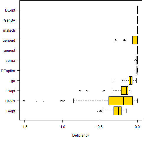

Figure 2: Difference in utility from optimal for all optimizers on the binding problem. 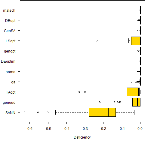We can characterize the results as: evolutionary better than genetic better than simulated annealing.  With one big exception.  GenSA — which hails from simulated annealing land — does very well.

I’m guessing that genoud would have done better if the differentiation were applied only to the weights and not the first part of the solution vector.

The other thing of note is that DEoptim is a more robustly developed version of differential evolution than is DEopt.  However, DEopt outperforms DEoptim.  DEopt does not have box constraints, so its solution vectors grow in size as the algorithm progresses.  This seems to make the problem easier. A weakness of DEopt turned out to be a strength.

Figures 3 and 4 show the results for the six best optimizers — same picture, different scale.

Figure 3: Difference in utility from optimal for the best optimizers on the non-binding problem.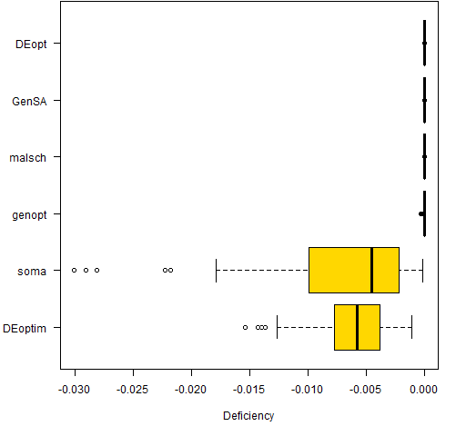

Figure 4: Difference in utility from optimal for the best optimizers on the binding problem.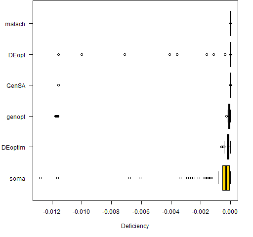

Update 2012/07/26

This update shows an advantage of heuristic algorithms that I was hoping I wouldn’t teach.

Randomization, for better or worse, often compensates for bugs.

— Jon Bentley More Programming Pearls (page 32)

Even though the code was not doing anything close to its intended behavior, the algorithms still managed to move towards the optimum.

Luca  Scrucca spotted that I used order when I meant rank.  I have re-run the race with the new version.  There are two changes in the new race:

• the right code makes it easier for the optimizers
• the new code is slower, so the optimizers get fewer evalations

I adjusted control arguments so that about a second on my machine would be used for each run.  Since rank is significantly slower than order in this case (see “R Inferno-ism: order is not rank”), only about one-quarter to one-third as many evaluations were allowed.

(By the way, I’m rather suspicious of the timings — they seem to jump around a bit too much.  It is a Windows machine.)

The new pictures are in Figures 5 and 6.

Figure 5: Difference in utility from optimal for all optimizers on the non-binding problem with the revised code.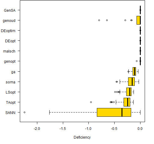 

Figure 6: Difference in utility from optimal for all optimizers on the binding problem with the revised code.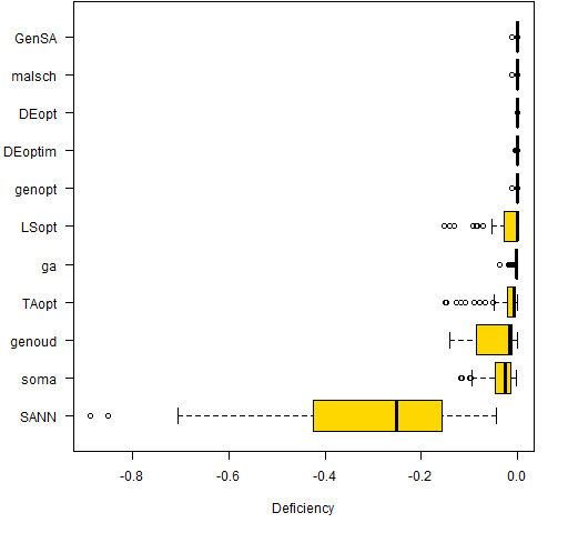

The results that look good in Figures 5 and 6 generally look good under a microscope as well — there are a lot of results that are essentially perfect.

The revised functions are in heuristicfuns_rev.R while the results from the second race are testresults10rev.R and the original results are testresults10.R.

Caveat

You should never (ever) think that you understand the merits of optimizers from one example.

I have no doubt that very different results could be obtained by modifying the control parameters of the optimizers.  In particular the results are highly dependent on the time allowed.  Some optimizers will be good at getting approximately right but not good at homing in on the exact solution — these will look good when little time is allowed.  Other algorithms will be slow to start but precise once they are in the neighborhood — these will look good when a lot of time is allowed.

For genetic and evolutionary algorithms there is a big interaction between time allowed and population size.  A small population will get a rough approximation fast.  A large population will optimize much slower but (generally) achieve a better answer in the end.

Exact circumstances are quite important regarding which optimizer is best.

Summary

If your problem is anything like this problem, then the Rmalschains and GenSA packages are worth test driving.

See also

• (update 2012 August 20) Another comparison of heuristic optimizers
• (update) genopt is now in the BurStMisc package on CRAN

Appendix R

The functions that ran the optimizers plus the code and data for the problems are in heuristic_objs.R.  (The 10a problem is non-binding and 10s is binding.)

The objective achieved by Portfolio for the non-binding problem is -0.38146061845033 and for the binding problem it is -1.389656885372.

In case you want to test routines on these problems outside R: the variance is in variance10.csv and the two expected return vectors are in expectedreturns10.csv.