We look at volatility clustering, and some aspects of modeling it with a univariate GARCH(1,1) model.

Volatility clustering

Volatility clustering — the phenomenon of there being periods of relative calm and periods of high volatility — is a seemingly universal attribute of market data.  There is no universally accepted explanation of it. GARCH (Generalized AutoRegressive Conditional Heteroskedasticity) models volatility clustering.  It does not explain it.  Figure 1 is an example of a garch model of volatility.

Figure 1: S&P 500 volatility until late 2011 as estimated by a garch(1,1) model. 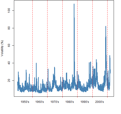Clearly the volatility moves around through time.  Figure 1 is a model of volatility, not the true volatility.  But if we had a picture of the true volatility, it would look remarkably like Figure 1.

Data demands

The natural frequency of data to feed a garch estimator is daily data.  You can use weekly or monthly data, but that smooths some of the garch-iness out of the data.

You can use garch with intraday data, but this gets complicated.  There is seasonality of volatility throughout the day.  The seasonality highly depends on the particular market where the trading happens, and possibly on the specific asset.  One particular example of such messiness looks at intraday Value at Risk.

How much daily data should you give garch?  In some respects the answer is: “more than you have”.  There’s a reason for that.

Figure 1 does not show true volatility because we never observe volatility.  Volatility ever only indirectly exposes itself to us.  So we are trying to estimate something that we never see.

Figure 2 is a sketch of a prototypical garch model.

Figure 2: Sketch of a “noiseless” garch process.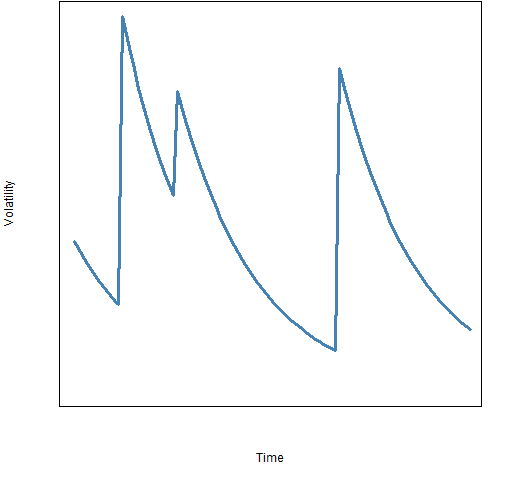

The garch view is that volatility spikes upwards and then decays away until there is another spike.  It is hard to see that behavior in Figure 1 because time is so compressed, it is more visible in Figure 3.

Figure 3: Volatility of MMM as estimated by a garch(1,1) model.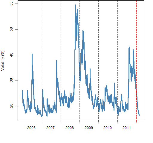

Of course in the real data there are shocks of all sizes, not just big shocks.

Note that volatility from announcements (as opposed to shocks) goes the other way around — volatility builds up as the announcement time approaches, and then goes away when the results of the announcement are known.

The estimation of a garch model is mostly about estimating how fast the decay is.  The decay that it sees is very noisy, so it wants to see a lot of data.  Lots of data as in it would like tens of thousands of daily observations.

There are two reasons not to give it tens of thousands of observations:

• you don’t have tens of thousands of observations
• markets change through time

So there is a balancing act.  2000 daily observations tends to be not unreasonable.

If you have less than about 1000 daily observations, then the estimation is unlikely to give you much real information about the parameters.  It is probably better to just pick a “reasonable” model.  That is going to be one with about the right persistence (see below), with the alpha1 parameter somewhere between 0 and 0.1, and the beta1 parameter between 0.9 and 1.

Estimation

We are staying with a GARCH(1,1) model; not because it is the best — it certainly is not.  We are staying with it because it is the most commonly available, the most commonly used, and sometimes good enough.

Garch models are almost always estimated via maximum likelihood.  That turns out to be a very difficult optimization problem.  That nastiness is just another aspect of us trying to ask a lot of the data.  Assuming that you have enough data that it matters, even the best implementations of garch bear watching in terms of the optimization of the likelihood.

We know that returns do not have a normal distribution, that they have long tails.  It is perfectly reasonable to hypothesize that the long tails are due entirely to garch effects, in which case using a normal distribution in the garch model would be the right thing to do.  However, using the likelihood of a longer tailed distribution turns out to give a better fit (almost always).  The t distribution seems to do quite well.

Autocorrelation

If the volatility clustering is properly explained by the model, then there will be no autocorrelation in the squared standardized residuals.  It is common to do a Ljung-Box test to test for this autocorrelation.

Below is output for such tests (actually Box-Pierce in this case) on a fit assuming a normal distribution on returns for MMM:

Q-Statistics on Standardized Squared Residuals
------------------------------------
      statistic p-value
Lag10     2.973  0.9821
Lag15     5.333  0.9889
Lag20     6.532  0.9980

If you are used to looking at p-values from goodness of fit tests, you might notice something strange.  The p-values are suspiciously close to 1.  The tests are saying that we have overfit 1547 observations with 4 parameters.  That is 1547 really noisy observations.  I don’t think so.

A better explanation is that the test is not robust to this extreme data, even though the test is very robust.  It is probably counter-productive to test the squared residuals this way.  An informative test is on the ranks of the squared standardized residuals.

Persistence

The persistence of a garch model has to do with how fast large volatilities decay after a shock. For the garch(1,1) model the key statistic is the sum of the two main parameters (alpha1 and beta1, in the notation we are using here).

The sum of alpha1 and beta1 should be less than 1.  If the sum is greater than 1, then the predictions of volatility are explosive — we’re unlikely to believe that.  If the sum is equal to 1, then we have an exponential decay model.

It is possible to express the persistence as a half-life.  The half-life is log(0.5)/log(alpha1 + beta1), where the units will be the frequency of the returns.  When alpha1+beta1 hits 1, the half-life becomes infinite.

Why would we get estimates with infinite persistence?  The persistence is estimated by seeing how fast the decay looks during the in-sample period.  If there is a trend in the volatility during the in-sample period, then the estimator “thinks” that it never sees a full decay.  The shorter the sample period, the more likely there’s a trend that will fool the estimation.

The in-sample estimates of volatility will look quite similar no matter what the parameter estimates are.  Figures 1 and 3 would not change much if we changed the parameter estimates for the respective models.  But the parameters matter a lot when we are predicting out of sample.

Usefulness

Garch models are useful because of two things:

• you can predict with garch models
• you can simulate with garch models

Prediction

The farther ahead you predict, the closer to perfect your model has to be.  Garch models are not especially close to perfect.  If you are predicting with a time horizon of a month or more, then I’d be shocked if you got much value from a garch model versus a more mundane model.  If you are predicting a few days ahead, then garch should be quite useful.

The persistence of the model is a key driver of the predictions — it determines how fast the predictions go to the unconditional volatility.  If there really is a lot of persistence in the volatility and your model accurately captures the persistence, then you will get good predictions far ahead.

There are two different things that might be predicted:

• the volatility at each time point of the prediction period
• the average volatility from the start of the period to each time point in the period (often called the term structure)

For example, the volatility that goes into an option price is the average volatility until expiry, not the volatility on the expiry date.

So there are two things you need to know when predicting:

• which prediction do you want
• which prediction are you getting

Simulation

A garch simulation needs:

• a garch model (including the parameter values)
• a volatility state for the model
• a distribution of standardized (variance 1) innovation values

Almost always the volatility state that we want is the state at the end of the data.  That is, now.  We want to use the current state of volatility and peek into the future.

Using the empirical distribution — the standardized residuals from the fitted model — is often the best choice for the innovations.   The assumption of the distribution when fitting the model does have an influence even when using the empirical distribution.

The estimation procedure “tries” to make the residuals conform to the hypothesized distribution.  The standardized residuals from a model assuming a normal distribution will be closer to normally distributed than the residuals from a model on the same data assuming a t distribution.

Simulation is dependent on the estimated parameters, but not as seriously as with prediction.  Model errors compound as we simulate farther into the future, but they compound with a vengeance when we predict far into the future.

R packages

There are several choices for garch modeling in R.  None are perfect and which to use probably depends on what you want to achieve.  However, rugarch is probably the best choice for many.

I haven’t extensively used any of the packages — consider the remarks here as first impressions.

rugarch

This has the idea of a specification for a model that is a separate object.  Then there are functions for fitting (that is, estimating parameters), predicting and simulation.

Here is an example of fitting with a Student t distribution:

> gspec.ru <- ugarchspec(mean.model=list(
      armaOrder=c(0,0)), distribution="std")
> gfit.ru <- ugarchfit(gspec.ru, sp5.ret[,1])
> coef(gfit.ru)
          mu        omega       alpha1        beta1        shape 
7.300187e-04 2.266325e-06 6.911640e-02 9.272781e-01 4.194994e+00 
> # plot in-sample volatility estimates
> plot(sqrt(252) * gfit.ru@fit$sigma, type='l')

The optimization in this package is perhaps the most sophisticated and trustworthy among the packages that I discuss.

fGarch

fGarch is a part of the Rmetrics suite.

We’ll fit the same Student t model as above:

> gfit.fg <- garchFit(data=sp5.ret[,1], cond.dist="std")
> coef(gfit.fg)
          mu        omega       alpha1        beta1        shape 
7.263209e-04 2.290834e-06 6.901898e-02 9.271553e-01 4.204087e+00
> # plot in-sample volatility estimates
> plot(sqrt(252) * gfit.fg@sigma.t, type="l")

tseries

I believe that this package was the first to include a publicly available garch function in R.  It is restricted to the normal distribution.

> gfit.ts <- garch(sp5.ret[,1])
> coef(gfit.ts)
          a0           a1           b1 
6.727470e-06 5.588495e-02 9.153086e-01 
> # plot in-sample volatility estimates
> plot(sqrt(252) * gfit.ts$fitted.values[, 1], type="l")

bayesGARCH

I think Bayes estimation of garch models is a very natural thing to do.  We have fairly specific knowledge about what the parameter values should look like.

The only model this package does is the garch(1,1) with t distributed errors.  So we are happy in that respect.

> gbayes <- bayesGARCH(sp5.ret[,1])

However, this command fails with an error.  The command does work if we give the returns in percent:

> gbayes <- bayesGARCH(sp5.ret[,1] * 100)

This can be an issue with maximum likelihood estimation as well.  There is at least one garch implementation that is much better at optimizing with percent returns rather than returns in their natural scale.  One test you can do on the optimization is to estimate the model on the returns in both scales and compare the results.

The bayesGARCH function, though, doesn’t give us an estimate.  It gives us a matrix with columns corresponding to the parameters and rows corresponding to the visits of a Markov Chain Monte Carlo.  This is, sort of, a sample from the (posterior) distribution of the parameters.

We can get a more useful analysis if we impose a constraint on the persistence.  We do that by creating a function for the constraint:

> persistenceCons
function(psi)
    {
      psi[2] + psi[3] < .9986
    }

This is saying that a half-life of more than two years is not plausible.  We then use that constraint:

> gbayesCons <- bayesGARCH(sp5.ret[,1] * 100, 
    control=list(addPriorConditions=persistenceCons))

Now we do a selection from the results (which may or may not be reasonable) and compute the half-lifes in our distribution:

> gbayesChain <- gbayesCons$chain1[-1:-2500,][c(TRUE,FALSE),]
> gbayesHalflife <- log(.5)/log(rowSums(gbayesChain[, 
     c("alpha1", "beta")]))

The result is then plotted.

Figure 3andOneHalf: Bayesian estimate of the half-life of MMM volatility.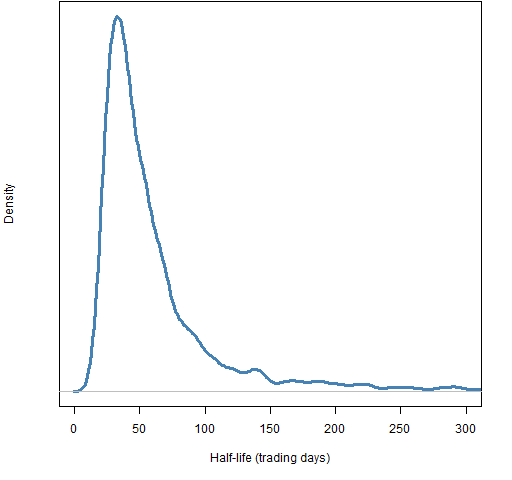

betategarch

This package fits an EGARCH model with t distributed errors.  EGARCH is a clever model that makes some things easier and other things harder.

> gest.te <- tegarch.est(sp5.ret[,1])
> gest.te$par
      delta        phi1      kappa1  kappa1star          df 
-0.05879721  0.98714860  0.03798604  0.02487405  4.50367108 
> gfit.te <- tegarch.fit(sp5.ret[,1], gest.te$par)
> pp.timeplot(sqrt(252) * gfit.te[, "sigma"] * 
     sd(gfit.te[,"epsilon"]))

That the plotting function is pp.timeplot is an indication that the names of the input returns are available on the output — unlike the output in the other packages up to here.  Figure 4 compares this estimate with a garch(1,1) estimate (from rugarch but they all look very similar).

Figure 4: Volatility of MMM as estimated by a garch(1,1) model (blue) and by the beta-t EGARCH model (gold).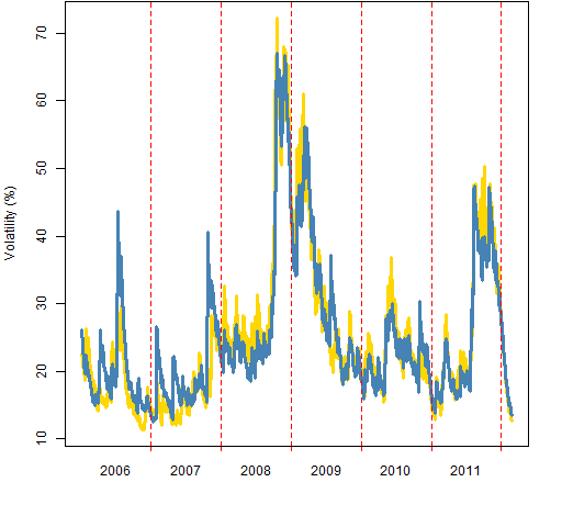

dynamo

I think the way to estimate a garch model in this package is:

gfit.dm <- dm(sp5.ret[,1] ~ garch(1,1))

But when I tried this command, it created a runtime error which ideally would have terminated R.  Instead R hung around doing whatever zombies do — dead and not wanting to go away.  Maybe it is the way to do it, but I don’t plan on trying it again for a while.

AutoSEARCH

This package will select an optimal lag (in some sense) for an ARCH model.  It has academic interest, but I’m doubtful of its usefulness in practice.

rgarch

This package is now obsolete: its descendants are rugarch and rmgarch.

More on R

• Another view is in “Which are my fave GARCH R packages …”.
• The CRAN finance task view is a good place to look for the current state

Questions

Have I mischaracterized any of the R packages?

Have I missed any R packages?

What good non-R implementations exist?

Updates

2012 July 06: Expanded the discussion of bayesGARCH beyond the first error and added a plot.  Corrected Figure 4 and the command that goes into it.  Added the AutoSEARCH package.

2012 September 24: There is a blog post on variance targeting (it seems to be a good idea).

2013 January 28: The components model is better than garch(1,1) and available in R.

2014 January 13: Some added explanation of garch that might help if some things in this post are confusing.