What is the difference between Monte Carlo — as it is usually defined in finance — and random portfolios?

The meaning of “Monte Carlo”

The idea of “Monte Carlo” is very simple.  It is a fancy word for “simulation”.

As usual, it is all too possible to find incredibly muddied explanations of such a simple concept.  For instance:

Monte Carlo is a mathematical model for computing the odds …

No.  Monte Carlo is a way of operating, not a model.  Monte Carlo (typically) uses a model to get results.  One Monte Carlo could use several models.

Monte Carlo is a general term, used across many fields of study.  In the personal finance sphere its meaning tends to be of projecting the value of a given portfolio into the future.

The meaning of “random portfolios”

Random portfolios as I use the term is a form of Monte Carlo, but quite distinct from the meaning we’ve seen.

Random portfolios are a sample from the set of portfolios that obey a given set of constraints.

Typically random portfolios are valued on historic data — though they may be generated before the valuation period takes place.

Importantly, random portfolios do not involve a model.  You may need to assume knowledge of the constraints, but random portfolios are rooted in reality.

The difference

Put succinctly:

• Monte Carlo creates hypothetical returns of a real portfolio
• Random portfolios are hypothetical portfolios using real asset returns

Example

Suppose we have a portfolio that consists of 100 shares each of MMM, AMD, CAT, FDX and XRX.  (In reality an equal-number-of-shares portfolio would be an indication of either bone-headed decision-making or a grandparent portfolio.)

Suppose further that it is the start of 2011 and we want to guess the value of our portfolio at the end of the year.  We can use Monte Carlo to do that. Figure 1 shows the weights of our portfolio on the last day of 2010.

Figure 1: Weights of the portfolio as of 2010-12-31.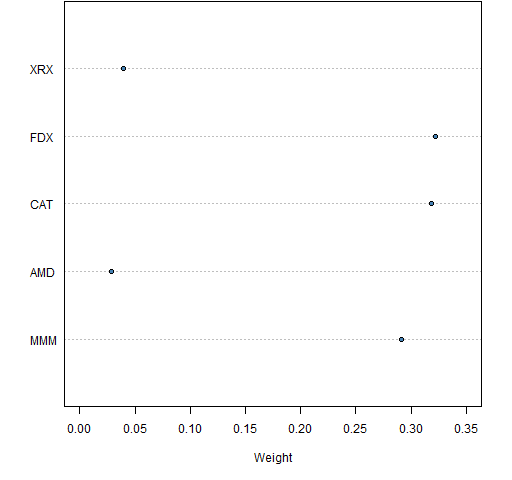
The traditional (and foolish) way to simulate the portfolio returns is to assume that the (log) returns are normally distributed.  One possible set of steps to do this is:

• estimate the mean vector and variance matrix for the daily returns of the assets
• do a large number of simulations of a year of daily returns
• calculate the portfolio return for each simulated year

Figure 2 shows the results from that type of simulation.

Figure 2: Monte Carlo distribution of predicted 2011 portfolio return assuming a normal distribution; the realized return is the vertical black line.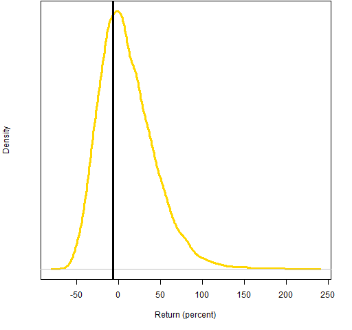

Note that this is a  portfolio of only 5 stocks, so we should expect it to be very volatile.

This simulation is terrible on many levels.  For example:

• returns are not normally distributed
• the simulation depends heavily on the mean returns over the estimation period
• it ignores the phenomenon of volatility clustering, and hence probably underestimates the probability of wild values

We can get rid of the normal distribution assumption by doing a simulation in the spirit of the statistical bootstrap.  Figure 3 shows the results of such a simulation.

Figure 3: Monte Carlo distribution of predicted 2011 portfolio return assuming empirical returns (blue) or a normal distribution (gold); the realized return is the vertical black line.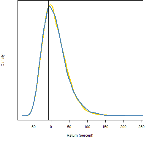

Relaxing the normality assumption has surprisingly little effect in this case.  (We are still assuming returns are independent — this assumption is wrong enough that it probably has a material effect.)

If we assume that the constraints on our portfolio are that it is long-only, the maximum weight is no more than 35% and there are at most 5 stocks in the portfolio, then we can generate a set of random portfolios (from the constituents of the S&P 500) that mimic our portfolio.  Figure 4 shows the distribution of the returns in 2011 for the random portfolios.

Figure 4: Distribution of 2011 returns for random portfolios with at most 5 names and maximum weight 35%; the realized return is the vertical black line. 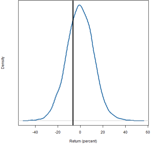The distribution in Figure 4 is drastically different from those in Figure 3.  That is because it is the distribution of a drastically different value.  The main difference is that it uses the price movements that actually happened in 2011 (rather than hypothesizing returns).  The other difference is that it is for multiple portfolios (rather than our single portfolio).

Figure 4 is saying that of the portfolios that meet the constraints, about 70% did better than our portfolio in 2011.

Monte Carlo resources

People that I know are doing research in this area:

• Michael Dempster at Cambridge Systems Associates
• Jarrod Wilcox

Other resources I’ve found (no guarantees — at all — on the quality of any of these):

• Vanguard Retirement nest egg calculator (simplistic, but rather fun)
• FIRECalc
• Standard and Poor’s Ameriprise calculator
• New York Times: A Planning Aid, but Not a Road Map
• CBS News: Retirement Calculator Report Card: Are You Saving Enough?
• Enjoy Retirement Jobs: Review of Retirement Calculators
• retirement planning calculators
• The flexible retirement planner
• Tipster from prospercuity

Questions

What resources have I missed?

What comments do you have on the resources I didn’t miss?

Summary

Monte Carlo is useful for personal investors to explore the adequacy of their savings.  Individual investors can (and should) perform Monte Carlo on their own portfolio.

The results of random portfolios are useful to individual investors in that they can indicate the amount of skill their fund managers have exhibited.  It is the fund managers rather than the individual investors that should be generating the random portfolios.

Thanks to Perry for prompting this post.

Epilogue

He’ll say you get just what you get
The simple truth is always the best
Don’t you see what’s done is done

from “The Facts about Jimmy” by Shawn Colvin & John Leventhal

Appendix R

the data

The data are computed from adjusted daily closing prices taken from Yahoo.  The matrix of returns that I have is called sp5.ret.

You can play around with fictionalized data by installing the pprobeData package:

install.packages("pprobeData",
   repos="https://www.portfolioprobe.com/"R)

If you are not on Windows, you will probably need to add the argument type="source".  Once you have installed the package on your machine, you need to add it to each R session in which you want to use it — do that with:

require(pprobeData)

portfolio returns

The exact computation of portfolio returns over time typically involves both log returns and simple returns, as explained in “A tale of two returns”.

Here is a function that takes a matrix of daily log asset returns and the initial portfolio weights.

> pp.porteval
function (dlar, weight)
{
        (exp(colSums(dlar[, names(weight)])) - 1) %*%
              weight
}

normal simulation

The simulation assuming a normal distribution starts off with some estimation:

mcmean <- colMeans(sp5.ret[1:1258,names(mcport)])
mcvar <- var(sp5.ret[1:1258,names(mcport)])

Note that using the sample variance is okay in this case because we only have 5 assets.  If we were estimating the variance for a large number of assets, we would want a more sophisticated estimate of variance.

The function to do one simulation is:

> pp.normsim
function (exret, variance, weight, times=252)
{
        # require(MASS)
        dlar <- mvrnorm(times, exret, variance)
        pp.porteval(dlar, weight)
}

It is used like:

mcnorm <- numeric(1e4)
for(i in 1:1e4) mcnorm[i] <- pp.normsim(mcmean,
      mcvar, mcport.wt)

empirical simulation

The function to do one empirical simulation is

> pp.bootsim
function (retmat, weight, times=252)
{
        dlar <- retmat[sample(nrow(retmat), times,
             replace=TRUE),]
        pp.porteval(dlar, weight)
}

It is used as:

mcboot <- numeric(1e4)
for(i in 1:1e4) mcboot[i] <- pp.bootsim(sp5.ret[1:1258,
      names(mcport.wt)], mcport.wt

random portfolio generation

The Portfolio Probe software is needed to generate the random portfolios.  The commands to get the random portfolios and their returns was:

require(PortfolioProbe)
mcrand5 <- random.portfolio(1e4, 
    prices=sp5.close[1259,],
    gross=1e6, long.only=TRUE, port.size=5,
    max.weight=.35)
mcrand5.ret11 <- valuation(mcrand5, sp5.close[
    c(1259, 1511), ], returns='simple')

plotting

The density plots are produced like:

plot(density(mcboot * 100))