We come closer to a definitive answer on the relative merit of Ledoit-Wolf shrinkage versus a statistical factor model for variance matrices.

Previously

This post builds on the post entitled:

• A test of Ledoit-Wolf versus a factor model

That post depended on some posts previous to it.

New information

Previously we generated random portfolios with the risk fraction of all assets constrained to be no more than 5%.  That constraint was based on the Ledoit-Wolf variance.  For this post we generated two more sets of random portfolios:

• factor model risk fractions all no more than 5% per asset
• factor model and Ledoit-Wolf risk fractions all no more than 5% per asset

These were again generated as of the end of Q3 2008 and the realized volatility of the portfolios was found for Q4 of 2008.  The correlations between the predicted volatilities and the realized volatilities were:

• factor model risk fraction, factor model prediction: 78.8%
• factor model risk fraction, Ledoit-Wolf prediction: 79.7%
• both risk fractions, factor model prediction: 75.3%
• both risk fraction, Ledoit-Wolf prediction: 76.2%

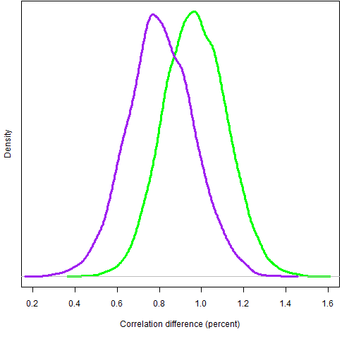
Again we bootstrapped the difference in correlations.  The bootstrap distributions of the correlation differences are shown in Figure 1.

Figure 1: Difference in correlations with risk fraction constraints on the factor model (green line) and on both variances (purple line).  Positive numbers mean Ledoit-Wolf is better.In both instances the Ledoit-Wolf correlation was larger than the factor model correlation for all bootstrap samples.

Summary

We’ve tested Ledoit-Wolf versus statistical factor model in four settings:

• weights constrained
• Ledoit-Wolf risk fractions constrained
• factor model risk fractions constrained
• Ledoit-Wolf risk fractions and factor model risk fractions constrained

In all four cases the Ledoit-Wolf predictions of volatility had a higher correlation with realized volatility than the corresponding factor model predictions.

In the case of weight constraints the difference in correlations was not statistically significant.  But in all of the other three cases the Ledoit-Wolf correlation was larger than the factor model correlation in all bootstrap samples.

It had been hypothesized that the Ledoit-Wolf prediction could have an unfair advantage when the constraints depended on the Ledoit-Wolf variance.  But that sort of bias doesn’t seem to exist.

In summary we now have clear evidence of Ledoit-Wolf outperforming the factor model.  This evidence is restricted to:

• this universe of stocks
• this time period

While the universe could theoretically be an important factor, that seems quite unlikely to me.

The time period could indeed be an issue.  In fact, the period was specially selected because it is unusual.  (However, it is an important case of unusual.)

Appendix R

Here are the R commands that did the computing to arrive at Figure 1.  First is to generate the random portfolios with the risk fraction constraints on the factor model variance.

require(PortfolioProbe)

rp.08Q3.rf05fm <- random.portfolio(1000, prices=sp500.price08Q3, gross=1e6, long.only=TRUE, risk.fraction=.05, port.size=c(40,50), variance=sp500.fmvar08Q3)

Next is to generate the random portfolios with risk fraction constraints on both variance matrices.  In preparation for that we create a two-column matrix of lower and upper constraints for the risk fractions.

sprf <- cbind(rep(-1,392), .05)
rownames(sprf) <- names(sp500.price08Q3)

You might think that the appropriate lower bound would be zero.  But risk fractions can be negative and we don’t  have anything against negative values appearing in this case (though the probability of that occurring is probably minuscule).

The command to generate the random portfolios uses the threeDarr function.  Something like this function is likely to appear in future versions of Portfolio Probe.  It takes some number of matrices and creates a three-dimensional array out of them.  The abind package (on CRAN) is a general tool in this regard.

rp.08Q3.rf05both <- random.portfolio(1000, prices=sp500.price08Q3, gross=1e6, long.only=TRUE, risk.fraction=threeDarr(sprf,sprf), port.size=c(40,50), variance=threeDarr(sp500.fmvar08Q3, sp500.var08Q3))

We get the predicted volatilities of each set of random portfolios with each variance matrix:

rp.08Q3.rf05fm.lwpvol <- sqrt(252 * unlist(randport.eval(rp.08Q3.rf05fm, keep='var.values', additional.args=list(variance=sp500.var08Q3))))

rp.08Q3.rf05fm.fmpvol <- sqrt(252 * unlist(randport.eval(rp.08Q3.rf05fm, keep='var.values', additional.args=list(variance=sp500.fmvar08Q3))))

rp.08Q3.rf05both.lwpvol <- sqrt(252 * unlist(randport.eval(rp.08Q3.rf05both, keep='var.values', additional.args=list(variance=sp500.var08Q3, risk.fraction=NULL))))

rp.08Q3.rf05both.fmpvol <- sqrt(252 * unlist(randport.eval(rp.08Q3.rf05both, keep='var.values', additional.args=list(variance=sp500.fmvar08Q3, risk.fraction=NULL))))

Next compute the valuations of the random portfolios for each day in the fourth quarter and use those to get the realized volatilities.

rp.08Q3.rf05fm.Q4val <- valuation(rp.08Q3.rf05fm, prices=as.matrix(sp500.closeok[440:504,]), collapse=TRUE)

rp.08Q3.rf05both.Q4val <- valuation(rp.08Q3.rf05both, prices=as.matrix(sp500.closeok[440:504,]), collapse=TRUE)

rp.08Q3.rf05fm.Q4vol <- sqrt(252) * sd(na.omit(diff(log(rp.08Q3.rf05fm.Q4val))))

rp.08Q3.rf05both.Q4vol <- sqrt(252) * sd(na.omit(diff(log(rp.08Q3.rf05both.Q4val))))

Now we’re in a position to bootstrap correlations.

boot.rf05fm.ledwolf <- numeric(10000)
boot.rf05fm.facmod <- numeric(10000)
boot.rf05both.ledwolf <- numeric(10000)
boot.rf05both.facmod <- numeric(10000)

for(i in 1:10000) {
the.samp <- sample(1000, 1000, replace=TRUE)
boot.rf05fm.ledwolf[i] <- cor(rp.08Q3.rf05fm.lwpvol[the.samp], rp.08Q3.rf05fm.Q4vol[the.samp])

boot.rf05fm.facmod[i] <- cor(rp.08Q3.rf05fm.fmpvol[the.samp], rp.08Q3.rf05fm.Q4vol[the.samp])

boot.rf05both.ledwolf[i] <- cor(rp.08Q3.rf05both.lwpvol[the.samp], rp.08Q3.rf05both.Q4vol[the.samp])

boot.rf05both.facmod[i] <- cor(rp.08Q3.rf05both.fmpvol[the.samp], rp.08Q3.rf05both.Q4vol[the.samp])
}

Finally we can look at plots.  Like:

plot(density(boot.rf05fm.ledwolf - boot.rf05fm.facmod))

Subscribe to the Portfolio Probe blog by Email